Show code cell content
import mmf_setup; mmf_setup.nbinit()
import os
from pathlib import Path
import logging
logging.getLogger("matplotlib").setLevel(logging.CRITICAL)
logging.getLogger('numba').setLevel(logging.CRITICAL)
logging.getLogger('OMP').setLevel(logging.CRITICAL)
%matplotlib inline
import numpy as np, matplotlib.pyplot as plt
This cell adds /home/docs/checkouts/readthedocs.org/user_builds/iscimath-583-fractals/checkouts/latest/src to your path, and contains some definitions for equations and some CSS for styling the notebook. If things look a bit strange, please try the following:
- Choose "Trust Notebook" from the "File" menu.
- Re-execute this cell.
- Reload the notebook.
Solution 11: Brownian Motion (Random Walks)#
Here we present a partial solution of Assignment 11: Brownian Motion (Random Walks). For details about Brownian motion and random walks, please see the following (part of my Standard Model course):
The assignment asks you to consider Brownian motion where the steps \(x_n\) are independent and identically and independently distributed (iid) with some probability density function bracket (PDF) \(p(x)\). The distribution \(p_N(X)\) after \(N\) steps is simply the distribution obtained by summing \(N\) random variables \(x\) with PDF \(p(x)\). As discussed in Renormalizing Random Walks, the PDF of the sum of random variables is simply the convolution of the individual PDFs. This means that the Fourier transform of \(p_N(X)\) is just the Fourier transform of \(p(x)\) raised to the \(N\)th power.
For the gaussian distribution this is simple:
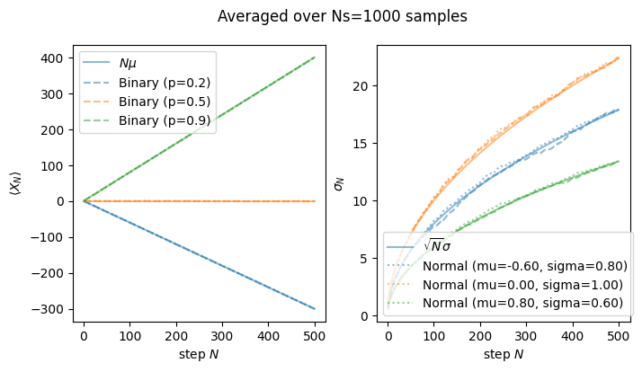
Thus, the position after \(N\) steps \(X_{N}\) is normally distributed with mean \(N\mu\) and standard deviation \(\sigma_N = \sqrt{N}\sigma\):
For the binary walk, the number of ways of ending up at position \(X_N = m-n\) is the number of ways of choosing \(m\) steps to be \(+1\) and \(n = N-m\) steps to be \(-1\). This gives the binomial distribution scaled by 2 and shifted by \(-N\)
whose mean and standard deviation are:
This gives the answer about how to relate the binary random walk and the gaussian random walk:
Another Approach
We can follow the same approach we used for a gaussian, considering the Fourier transform of the binary distribution:
Expanding for small \(k\) we have:
as stated above.
Show code cell source
def get_binary_walk(N, p=0.5, seed=2):
    """Return a binary random walk of N steps."""
    rng = np.random.default_rng(seed=seed+10)

    # Slight trick: we get a binary distribution from the uniform
    # distribution on [0, 1].
    dx = np.where(rng.uniform(size=N) < p, 1, -1)
    x = np.cumsum(dx)
    return x

def get_normal_walk(N, mean=0, stdev=1, seed=2):
    """Return a gaussian random walk of N steps."""
    rng = np.random.default_rng(seed=seed+10)
    dx = rng.normal(loc=mean, scale=stdev, size=N)
    x = np.cumsum(dx)
    return x

ps = [0.2, 0.5, 0.9]

fig, axs = plt.subplots(1, 2, figsize=(4*2, 4))

N = 500
Ns = 1000
step = 1+np.arange(N)
for n, p in enumerate(ps):
    mu, sigma = 2*p-1, 2*np.sqrt(p*(1-p))
    x_bs = np.array([get_binary_walk(N, p=p, seed=n)
                     for n in range(Ns)])
    x_ns = np.array([get_normal_walk(N, mean=mu, stdev=sigma, seed=n)
                     for n in range(Ns)])
    kw = dict(c=f"C{n}", alpha=0.5)
    label = r"$N \mu $" if n == 0 else None
    axs[0].plot(step, step*mu, '-', label=label, **kw)
    axs[0].plot(step, x_bs.mean(axis=0), '--', label=f"Binary ({p=})", **kw)
    axs[0].plot(step, x_ns.mean(axis=0), ':', **kw)

    label = r"$\sqrt{N}\sigma$" if n == 0 else None
    axs[1].plot(step, np.sqrt(step)*sigma, '-', label=label, **kw)
    axs[1].plot(step, x_bs.std(axis=0), '--', **kw)
    axs[1].plot(step, x_ns.std(axis=0), ':', label=f"Normal ({mu=:.2f}, {sigma=:.2f})", **kw)
axs[0].set(xlabel="step $N$", ylabel=r"$\langle X_N \rangle$");
axs[1].set(xlabel="step $N$", ylabel=r"$\sigma_N$");
axs[0].legend()
axs[1].legend()
plt.suptitle(f"Averaged over {Ns=} samples");