Show code cell content
import mmf_setup; mmf_setup.nbinit()
import os
from pathlib import Path
import logging
logging.getLogger("matplotlib").setLevel(logging.CRITICAL)
logging.getLogger('numba').setLevel(logging.CRITICAL)
logging.getLogger('OMP').setLevel(logging.CRITICAL)
%matplotlib inline
import numpy as np, matplotlib.pyplot as plt
This cell adds /home/docs/checkouts/readthedocs.org/user_builds/iscimath-583-fractals/checkouts/latest/src to your path, and contains some definitions for equations and some CSS for styling the notebook. If things look a bit strange, please try the following:
- Choose "Trust Notebook" from the "File" menu.
- Re-execute this cell.
- Reload the notebook.
Solution 10: Fractal Dimension of Julia Sets#
What is the fractal dimension of the Julia set \(J_{N g(z)}\) corresponding to Newton’s method for finding the roots of \(g(z) = z^3 - 1\)? This is the Julia set corresponding to the function
The box-counting dimension \(d\) relates the linear size \(\epsilon\) of the cells \(A = \epsilon^2\) to the number of cells in the Julia set \(N(\epsilon) \propto \epsilon^{-d}\) so that
First we define some code to get the boxes that contain points from the Julia set. We do this as follows:
First we construct a grid with \(N_{G} = 2^{G} + 1\) point in each direction. This allows use to recursively analyze nested subgrids of size \(N_{n} = 2^{n}+1\) for \(n\in \{0, 1, \cdots, N\}\). Combined with the extents \(L\) of the region, we can compute \(\epsilon = L/N_{N}\). (In higher dimension, we take the geometric mean, i.e. \(\epsilon = \sqrt{\d{x} \d{y}}\).)
We then iterate each point on the grid with \(z\mapsto f(z)\) until \(\abs{g(z)} < 0.9\). (See the discussion at the bottom for why this value works.)
We assign to each point on the grid an integer \(0\), \(1\), or \(2\), depending on which root is closest.
We treat these points as the boundaries of the cells, and claim that the cell contains points from \(J\) is the 4 boundary points are not all attracted to the same attractor. (Technically, we do this by taking the differences with
np.diffand checking if any of the differences is non-zero.)We repeat this for all subgrids, counting how many cells \(N(\epsilon)\) there are of “length” \(\epsilon\), then fitting a line to the logarithms to extract the dimension.
Show code cell source
def g(z):
    return z**3 -1

def f(z):
    # Little trick using masked arrays to prevent 1/0 errors.
    # We fill these values with 0 so that the point at z=0 stays there rather than
    # diverging to np.inf where it raises floating point warning.
    return 2/3*z + np.ma.divide(1, 3*z**2).filled(0)

roots = np.exp(2j*np.pi / 3 * np.arange(3))
assert np.allclose(g(roots), 0)

def get_closest_root(z, maxiter=20, roots=roots):
    for n in range(maxiter):
        z = f(z)
    closest_root = np.argmin(abs(z[:, :, None] - roots[None, None, :]), axis=-1)
    return closest_root

def get_J(attractor):
    """Return boolean array of cells containing points in J."""
    corners = np.array([
        attractor[:-1, :-1],
        attractor[:-1, 1:],
        attractor[1:, :-1],
        attractor[1:, 1:]])
    inside = abs(np.diff(corners, axis=0)).max(axis=0) > 0
    return inside


def get_counts(z0, R, G=10, maxiter=30, ax=None):
    """Return `(epss, Ns)` box-counting the Newton fractal.

    See analyze for argument description.

    Returns
    -------
    epss : list(float)
        List of the 1D cell lengths.
    Ns : list(int)
        Corresponding list of cell counts.
    """
    N = 2**G + 1
    x = np.linspace(z0.real-R, z0.real+R, N)
    y = np.linspace(z0.imag-R, z0.imag+R, N)
    z = x[:, None] + 1j*y[None, :]

    attractor = get_closest_root(z, maxiter=maxiter)

    epss = []
    Ns = []
    for n in 2**np.arange(0, G+1)[::-1]:  # Reverse the order - large cells to small.
        J = get_J(attractor[::n, ::n])
        x_, y_ = x[::n], y[::n]
        epss.append(np.sqrt(np.diff(x_).mean() * np.diff(y_).mean()))
        Ns.append(J.sum())

        if ax is not None:
            ax.pcolormesh(x_, y_, J.T, alpha=0.1)

    if ax is not None:
        ax.set(aspect=1, xlabel="$x=\Re z$", ylabel="$y=\Im z$");

    epss, Ns = np.array(epss), np.array(Ns)
    return epss, Ns


def analyze(z0=0, R=1, G=10, maxiter=10, skip=5, plot=True):
    """Plot an extract the dimension.

    Arguments
    ---------
    z0 : complex
        Center of outer box.
    R : float
        "Radus" of the outer box, which will be a square +-R centered on z0.
    G : int
        Largest grid will have `2**G + 1` points.
    maxiter : int
        Maximum number of iterations.
    skip : int
        Number of largest subgrids to skip when computing the dimenson.
    plot : bool
        If `True`, then plot.
    """
    if plot:
        fig, (ax, ax1) = plt.subplots(1, 2, figsize=(10, 5),
                                      gridspec_kw=dict(width_ratios=(2, 1)))
    else:
        ax = None
    epss, Ns = get_counts(z0=z0, R=R, G=G, maxiter=maxiter, ax=ax)

    dim, b = np.polyfit(np.log(1/epss)[skip:], np.log(Ns)[skip:], deg=1)
    if plot:
        ax1.loglog(1/epss, Ns, '+-')
        ax1.plot(1/epss, np.exp(np.polyval([dim, b], np.log(1/epss))))
        ax1.set(xlabel="Inverse cell length $1/\epsilon$", ylabel="$N$",
                title=f"dim = {dim:}")
    return dim
Here we apply these to the Newton fractal for \(g(z) = z^3 - 1\):
%time analyze(z0=0, R=1.25)
CPU times: user 505 ms, sys: 144 ms, total: 648 ms
Wall time: 647 ms
1.390608223180251
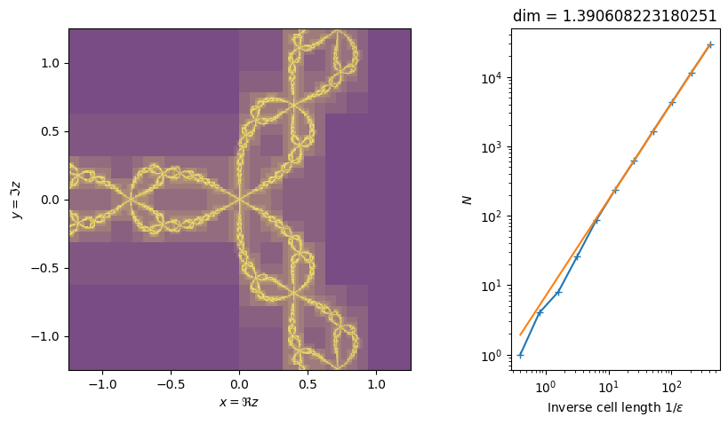
It seems like the box-counting dimension is about \(d = 1.4\). Let’s try zooming in.
%time analyze(z0=0, R=0.1)
CPU times: user 479 ms, sys: 120 ms, total: 599 ms
Wall time: 598 ms
1.0110880329215637
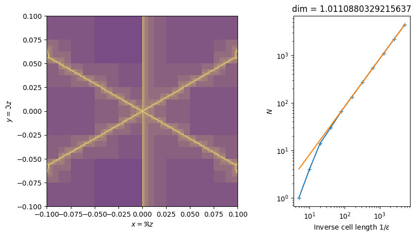
Hmm. This looks strange. If we zoom in, the dimension seems to drop. After playing a
bit, I found that the issues was my default choice of maxiter. Increasing this fixes
the issue.
Warning
You should always check that your results are converged! In this case, you should vary
maxiter and G, making sure that your results do not depend on these parameters. If
there is a significant dependence, then you must consider another method, or figure out
the nature of this dependence so you can extrapolate to the limits of large G and maxiter.
%time analyze(z0=0, R=0.1, maxiter=100)
CPU times: user 3.06 s, sys: 628 ms, total: 3.68 s
Wall time: 3.68 s
1.4394713267422707

Zooming out has a similar issue. Increasing maxiter fixes this again.
analyze(z0=0, R=100)
%time analyze(z0=0, R=100, maxiter=100)
CPU times: user 3.07 s, sys: 7.94 ms, total: 3.08 s
Wall time: 3.08 s
1.4343327137206128

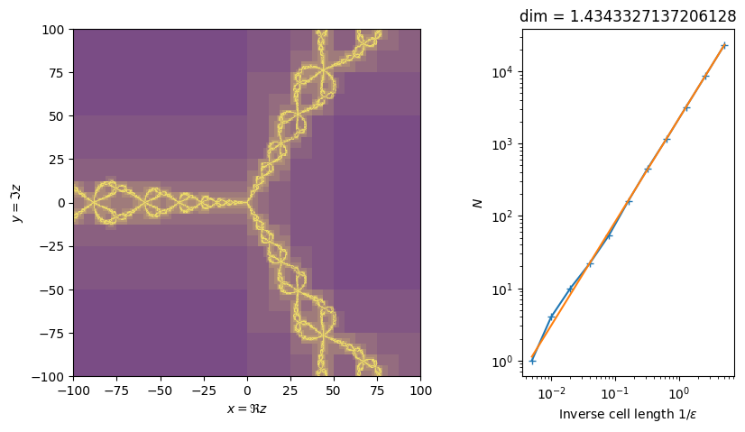
Apparently this Newton fractal is a multifractal (see [Nauenberg and Schellnhuber, 1989] for details). I expected that this meant that different regions of the Julia set might therefore have different dimensions. To check this, we zoom in off the axis:
%time analyze(z0=-0.63+0.2575j, R=0.001, maxiter=100)
CPU times: user 2.66 s, sys: 632 ms, total: 3.29 s
Wall time: 3.29 s
/tmp/ipykernel_4280/1532633877.py:92: RuntimeWarning: divide by zero encountered in log
  dim, b = np.polyfit(np.log(1/epss)[skip:], np.log(Ns)[skip:], deg=1)
1.4479895322548684

To within the precision of my analysis, I don’t see a significant variation here. Have you found anything? Perhaps the notion of a multifractal is more complicated.
Convergence Tests#
Here we perform some rudimentary convergence tests.
args = dict(z0=0, R=1.5, plot=False)
%time [analyze(maxiter=maxiter, **args) for maxiter in [10, 20, 30]]
CPU times: user 1.88 s, sys: 63.3 ms, total: 1.94 s
Wall time: 1.94 s
[1.411927491825257, 1.4475793909154753, 1.4476161276332395]
args['maxiter'] = 50
%time [analyze(G=G, **args) for G in [9, 10, 11]]
CPU times: user 7.41 s, sys: 3.38 s, total: 10.8 s
Wall time: 10.8 s
[1.448557390582579, 1.44753381893522, 1.4464607967320142]
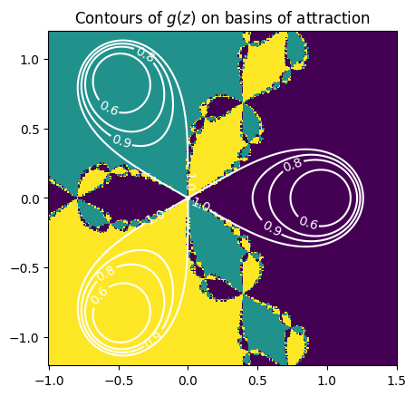
Speed Improvements#
By plotting some contours, we show that if \(\abs{g(z)} < 0.9\), then \(z\) lies in the basin of attraction for the nearest root. This allows us to loosen our effective cutoff criterion.
x = np.linspace(-1, 1.5, 256)
y = np.linspace(-1.2, 1.2, 256)
z = x[:, None] + 1j*y[None, :]

attractor = get_closest_root(z)

fig, ax = plt.subplots()
ax.pcolormesh(x, y, attractor.T)
cs = ax.contour(x, y, abs(g(z)).T, levels=[0.6, 0.8, 0.9, 1], colors='w')
ax.clabel(cs, cs.levels, inline=True)
ax.set(aspect=1, title="Contours of $g(z)$ on basins of attraction");
Here we code a vectorized version… Incomplete.