Show code cell content
import mmf_setup; mmf_setup.nbinit()
import os
from pathlib import Path
import logging
logging.getLogger("matplotlib").setLevel(logging.CRITICAL)
logging.getLogger('numba').setLevel(logging.CRITICAL)
logging.getLogger('OMP').setLevel(logging.CRITICAL)
%matplotlib inline
import numpy as np, matplotlib.pyplot as plt
This cell adds /home/docs/checkouts/readthedocs.org/user_builds/iscimath-583-fractals/checkouts/latest/src to your path, and contains some definitions for equations and some CSS for styling the notebook. If things look a bit strange, please try the following:
- Choose "Trust Notebook" from the "File" menu.
- Re-execute this cell.
- Reload the notebook.
Solution 7: Pseudo-Random Numbers#
Here is a partial solution to Assignment 7: Pseudo-Random Numbers. Recall that iterating \(x\mapsto 4x(1-x)\) seemed to give uniform random deviates for the variable
However, when used to generate the Sierpiński gasket with a Multiple Reduction Copy Machine (MRCM), this failed spectacularly. Here is the recap:
%matplotlib inline
import numpy as np, matplotlib.pyplot as plt
import scipy.stats, scipy as sp

plt.rcParams['figure.figsize'] = (5, 3)

def get_sierpinski(y):
    """Return samples in he Sierpinski gasket using the random numbers y."""

    # Fixed points in an equilateral triangle
    thetas = 2*np.pi * (np.arange(3)/3 + 1/4)
    ps = np.exp(1j*thetas)

    p = ps[0]   # Start with one point.
    ns = np.floor(3*y).astype(int)
    res = [p]
    for n in ns:
        p1 = ps[n]  # Choose one of the three points randomly
        p = (p + p1)/2  # Move half-way to p1.
        res.append(p)
    return np.array(res)

def get_random_x(N, x0=np.sqrt(2)):
    """Return N pseudo-random numbers between 0 and 1.

    Arguments
    ---------
    N : int
        Number of pseudo-random numbers to generate.
    x0 : float
        Seed to start the generator.  Must be chosen carefully.
    """
    x = x0 % 1  # The mod operator % makes sure initial point is 0 <= x0 < 1.
    xs = [x]
    while len(xs) < N:
        x = 4*x*(1-x)
        xs.append(x)
    return np.array(xs)

def get_uniform(N, x0=np.sqrt(2)):
    """Return N uniformly distributed numbers between 0 and 1."""
    x = get_random_x(N=N, x0=x0)
    y = 0.5 - np.arcsin(1-2*x)/np.pi
    return y
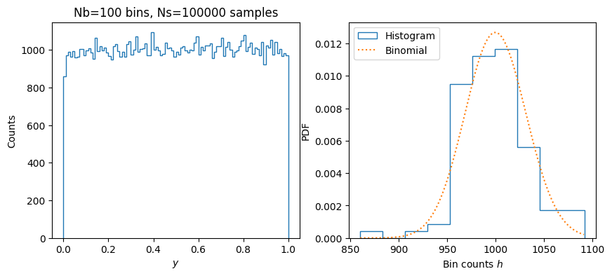
Nb = 100     # Number of bins equally spaced between 0 and 1
Ns = 100000  # Number of samples.
y = get_uniform(N=Ns)
h, bins = np.histogram(y, bins=Nb, range=(0, 1))  # Histogram

fig, axs = plt.subplots(1, 2, figsize=(10,4))
ax = axs[0]
ax.stairs(h, bins)
ax.set(xlabel="$y$", ylabel="Counts", title=f"{Nb=} bins, {Ns=} samples");

ax = axs[1]
ax.hist(h, bins=len(h)//10, density=True, histtype='step', label="Histogram")
ax.set(xlabel="Bin counts $h$", ylabel="PDF");

# This should be a binomial distribution.
rv = sp.stats.binom(Ns, p=1/Nb)
h_ = np.arange(h.min(), h.max())
ax.plot(h_, rv.pmf(h_), ':', label="Binomial")
ax.legend();
This looks good, but the Sierpiński gasket looks very bad. (To compare, we plot the version with NumPy’s random numbers underneath.)
rng = np.random.default_rng(seed=2)
p = get_sierpinski(y)
p_numpy = get_sierpinski(rng.random(len(y)))
fig, ax = plt.subplots()
ax.plot(p_numpy.real, p_numpy.imag, 'C1.', ms=0.5, label="NumPy")
ax.plot(p.real, p.imag, 'C0.', ms=0.5, label=r"$x \mapsto 4x(1-x)$")
ax.legend()
ax.set(aspect=1, xlabel="x", ylabel="y");
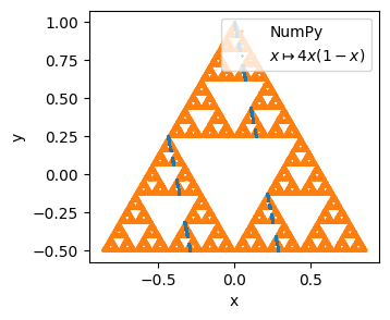
We see here that our algorithm never gets to the bottom right or bottom left points. To get to these points, we would need a long sequence of \(1\) or \(2\), but it turns out that we never get these with our generator.
from itertools import product

ns = np.floor(3*y).astype(int).tolist()  # Indices 0, 1, or 2
fig, axs = plt.subplots(1, 3, figsize=(10, 3))

ax = axs[0]
keys = sorted(set(ns))
counts = [ns.count(n) for n in keys]
ax.bar([str(key) for key in keys], counts)

ax = axs[1]
n2s = list(zip(ns, ns[1:]))
keys = list(product(*[(0, 1, 2)]*2))
counts = [n2s.count(n2) for n2 in keys]
ax.bar([''.join(map(str, key)) for key in keys], counts)

ax = axs[2]
n3s = list(zip(ns, ns[1:], ns[2:]))
keys = list(product(*[(0, 1, 2)]*3))
counts = [n3s.count(n3) for n3 in keys]
ax.bar([''.join(map(str, key)) for key in keys], counts)
plt.setp(ax.get_xticklabels(), rotation=90, size=8)
#ax.tick_params(axis='x', labelrotation=90, size=5)  # Size is ignored?
#plt.xticks(ha='right')  # Should be included above eventually
plt.tight_layout()
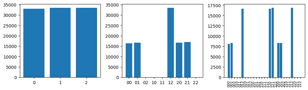
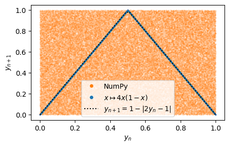
This clarifies why the Sierpinski gasket fails: certain combinations like 02, 10, 11, and 22 never appear. Specifically, our generator never produces orbits with successive 1’s or 2’s. In other words, successive numbers are not independent. After a little reflection, this should be obvious since \(y_{n+1} = 1-\abs{2y_{n}-1}\). We can see this by plotting \(y_{n+1}\) vs \(y_{n}\):
fig, ax = plt.subplots()
_y = rng.random(size=len(y))
ax.plot(_y[:-1], _y[1:], 'C1.', ms=0.2, label="NumPy")
ax.plot(y[:-1], y[1:], 'C0.', ms=0.2, label=r"$x\mapsto 4x(1-x)$")
_y = np.linspace(0, 1)
ax.plot(_y, 1-abs(2*_y-1), 'k:',label=r"$y_{n+1} = 1-|2y_{n}-1|$")
ax.legend(markerscale=40)
ax.set(xlabel="$y_{n}$", ylabel="$y_{n+1}$");
Improvements#
How can we improve our generator? One idea is to skip lag intermediate steps:
fig, ax = plt.subplots()
for lag in range(1, 5):
    ax.plot(y[:-lag], y[lag:], '.', ms=0.1)
ax.set(xlabel="$y_{n}$", ylabel="$y_{n+\mathrm{lag}}$",
       title=r"lag $\in \{1, 2, 3, 4\}$");
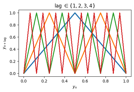
Geometrically the effect is obvious, folding the initial tent back on itself until it gradually fills the space. A little trial and error gives us an idea of how much lag is needed:
lags = [1, 2, 3, 4, 5, 6]
fig, axs = plt.subplots(1, len(lags), figsize=(len(lags)*2, 2))
Ns = 10000
for lag, ax in zip(lags, axs):
    y = get_uniform(lag*Ns)[::lag]
    p = get_sierpinski(y)
    ax.plot(p.real, p.imag, 'C0.', ms=0.1)#, label=r"{lag=}")
    ax.set(xlim=(-1,1), ylim=(-0.51, 1.01), aspect=1, title=f"{lag=}");
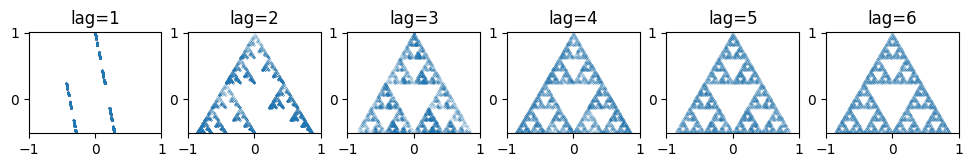
Note that this is quite wasteful since we discard lag points, but it seems to work
reasonably well.
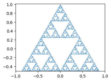
def get_random_x_lag(N, x0=np.sqrt(2), lag=10):
    """Return N pseudo-random numbers between 0 and 1 with lag."""
    x = x0 % 1
    xs = [x]
    while len(xs) < N:
        for n in range(lag):
            x = 4*x*(1-x)
        xs.append(x)
    return np.asarray(xs)

def get_uniform_lag(N, x0=np.sqrt(2), lag=10):
    x = get_random_x_lag(N, x0=x0, lag=lag)
    return 0.5 - np.arcsin(1-2*x)/np.pi

N = 10000
y = get_uniform_lag(N)
p = get_sierpinski(y)
fig, ax = plt.subplots()
ax.plot(p.real, p.imag, '.', ms=0.2)
ax.set(xlim=(-1,1), ylim=(-0.51, 1.01), aspect=1);
Further Issues#
Consider the following “improvement” where we directly iterate the tent map \(y \mapsto 1 - \abs{2y-1}\):
def get_uniform_lag2(N, x0=np.sqrt(2), lag=10):
    """Return N uniformly distributed numbers between 0 and 1."""
    y = 0.5 - np.arcsin(1-2*(x0 % 1))/np.pi
    ys = [y]
    while len(ys) < N:
        for n in range(lag):
            y = 1 - abs(2*y-1)
        ys.append(y)
    return np.asarray(ys)

N = 10000
y = get_uniform_lag2(N)
p = get_sierpinski(y)
fig, ax = plt.subplots()
ax.plot(p.real, p.imag, '.', ms=0.1)
ax.set(xlim=(-1,1), ylim=(-0.51, 1.01), aspect=1);
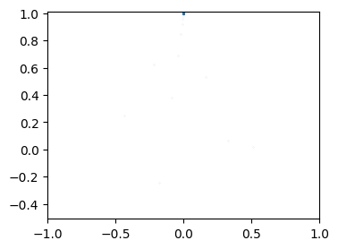
Formally, this does the same thing but obviously does not work in practice. Why? Let’s plot a few iterates and see.
N = 100
y1 = get_uniform_lag(N, lag=1)
y2 = get_uniform_lag2(N, lag=1)
fig, ax = plt.subplots()
ax.plot(y1, label=r"$x\mapsto 4x(1-x)$")
ax.plot(y2, label=r"$y\mapsto 1-|2y-1|$")
ax.legend()
<matplotlib.legend.Legend at 0x7f6ddcf89e10>
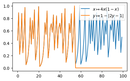
Notice that these match for about 52 iterations, after which the second iteration promptly falls to zero. [Schroeder, 1991] gives the key to this behaviour by noting that if we “flip” the meaning of \(y_{n+1} \rightarrow 1-y_{n+1}\) for \(y_{n}>1/2\), then the iteration becomes simply \(y \mapsto 2y \mod 1\). This is simply shifting the bits to the left by one and discarding the integer portion, thus, \(0.101011001 \mapsto 0.01011001 \mapsto 0.1011001 \cdots\). Since floating point numbers are represented on our computer in binary, with 52 digits of precision:
print(np.finfo(float))
Machine parameters for float64
---------------------------------------------------------------
precision =  15   resolution = 1.0000000000000001e-15
machep =    -52   eps =        2.2204460492503131e-16
negep =     -53   epsneg =     1.1102230246251565e-16
minexp =  -1022   tiny =       2.2250738585072014e-308
maxexp =   1024   max =        1.7976931348623157e+308
nexp =       11   min =        -max
smallest_normal = 2.2250738585072014e-308   smallest_subnormal = 4.9406564584124654e-324
---------------------------------------------------------------
after 52 shifts, we end up with exactly zero. Our initial algorithm thus relies on
round-off errors to keep providing non-zero iterations. This makes it very hard to
reproduce, since the exact sequence of numbers may depend on the implementation of
functions like np.arcsin and the hardware floating-point implementation.
Platform independent pseudo-random number generators generally use exact integer representations. For a good discussion and some algorithms, see [Press et al., 2007] and https://www.pcg-random.org/. The latter describes the PCG family which is now used in NumPy.