Show code cell content
import mmf_setup; mmf_setup.nbinit()
import os
from pathlib import Path
FIG_DIR = Path(mmf_setup.ROOT) / '../Docs/_build/figures/'
os.makedirs(FIG_DIR, exist_ok=True)
import logging; logging.getLogger("matplotlib").setLevel(logging.CRITICAL)
%matplotlib inline
import numpy as np, matplotlib.pyplot as plt
try: from myst_nb import glue
except: glue = None
This cell adds /home/docs/checkouts/readthedocs.org/user_builds/iscimath-583-fractals/checkouts/latest/src to your path, and contains some definitions for equations and some CSS for styling the notebook. If things look a bit strange, please try the following:
- Choose "Trust Notebook" from the "File" menu.
- Re-execute this cell.
- Reload the notebook.
Chaos and Feigenbaum’s Constant#
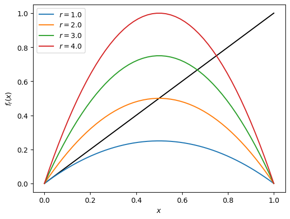
Here we consider the phenomena of period doubling in chaotic systems, which leads to universal behavior [Feigenbaum, 1978]. The quintessential system is that of the Logistic map:
which is a crude model for population growth. The interepretation is that \(r\) is proportional to the growth rate, and that \(x \in [0,1]\) is the total population as a fraction of the carrying capacity of the environment. For small \(x\), the population grows exponentially without bound \(x \mapsto r x\), while for large \(x \approx 1\) the population rapidly declines as the food is quickly exhausted and individuals starve.
def f(x, r, d=0):
    """Logistic growth function (or derivative)"""
    if d == 0:
        return r*x*(1-x)
    elif d == 1:
        return r*(1-2*x)
    elif d == 2:
        return -2*r
    else:
        return 0
Show code cell source
x = np.linspace(0, 1)

fig, ax = plt.subplots()
ax.plot(x, x, '-k')
for r in [1.0, 2.0, 3.0, 4.0]:
    ax.plot(x, f(x, r=r), label=f"$r={r}$")
ax.legend()
ax.set(xlabel="$x$", ylabel="$f_r(x)$");
The behaviour of this system is often demonstrated with a cobweb plot:
from math_583.plotting import CobWeb

c = CobWeb(f)

# Animate r from 1 to 4 but slow rs as they approach 4 since lots happens there.
rs = 1 + (4-1)*(1 - np.exp(-5*np.linspace(0, 1, 100)))
%time c.animate(rs=rs)
---------------------------------------------------------------------------
AttributeError                            Traceback (most recent call last)
File <timed eval>:1

File ~/checkouts/readthedocs.org/user_builds/iscimath-583-fractals/checkouts/latest/src/math_583/plotting.py:111, in CobWeb.animate(self, rs, interval_ms)
    109     x = np.sin(np.linspace(0.0, 1.0, 100) * np.pi / 2)
    110     rs = 1.0 + 3.0 * x
--> 111 animation = FuncAnimation(
    112     self.fig,
    113     self.cobweb,
    114     frames=rs,
    115     interval=interval_ms,
    116     init_func=self.init_func,
    117     blit=True,
    118 )
    119 display(HTML(animation.to_jshtml()))
    120 plt.close("all")

File ~/checkouts/readthedocs.org/user_builds/iscimath-583-fractals/conda/latest/lib/python3.11/site-packages/matplotlib/animation.py:1695, in FuncAnimation.__init__(self, fig, func, frames, init_func, fargs, save_count, cache_frame_data, **kwargs)
   1692 # Needs to be initialized so the draw functions work without checking
   1693 self._save_seq = []
-> 1695 super().__init__(fig, **kwargs)
   1697 # Need to reset the saved seq, since right now it will contain data
   1698 # for a single frame from init, which is not what we want.
   1699 self._save_seq = []

File ~/checkouts/readthedocs.org/user_builds/iscimath-583-fractals/conda/latest/lib/python3.11/site-packages/matplotlib/animation.py:1416, in TimedAnimation.__init__(self, fig, interval, repeat_delay, repeat, event_source, *args, **kwargs)
   1413 # If we're not given an event source, create a new timer. This permits
   1414 # sharing timers between animation objects for syncing animations.
   1415 if event_source is None:
-> 1416     event_source = fig.canvas.new_timer(interval=self._interval)
   1417 super().__init__(fig, event_source=event_source, *args, **kwargs)

AttributeError: 'NoneType' object has no attribute 'canvas'
Notice that as the growth constant increases, the population first stabilizes on a single fixed-point, but then this expands into a cycle of period 2, then a cycle of period 4 etc. This is called period doubling, and this behaviour can be summarized in a bifircation diagram.
Bifurcation Diagrams#
Here we develop an algorithm for drawing a high-quality bification diagram. We start with a simple algorithm that simply accumulates \(N\) iterations starting with \(x_0 = 0.2\) at a set of \(N_r\) points between \(r_0=2.0\) and \(r_1=4.0\).
fig, ax = plt.subplots()

r0 = 2.0
r1 = 4
Nr = 500
N = 200
x0 = 0.2

rs = np.linspace(r0,r1,Nr)
for r in rs:
    x = x0
    xs = []
    for n in range(N):
        x = f(x, r=r)
        xs.append(x)
    ax.plot([r]*len(xs), xs, '.', ms=0.1, c='k')
ax.set(xlabel='$r$', ylabel='$x$');
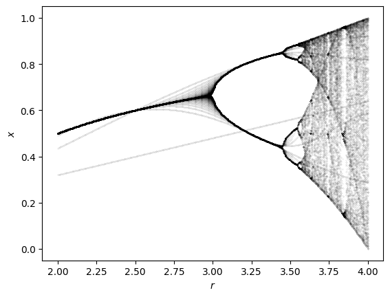
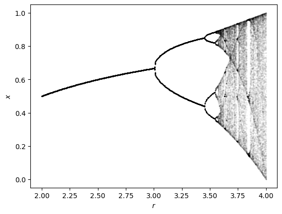
This works reasonably well, but has several artifacts. First, note the various curves - these are reminants of the choice of the initial point. Instead, we should iterate through some \(N_0\) iterations to allow the system to stabilize, then start accumulating.
fig, ax = plt.subplots()

N0 = 100

rs = np.linspace(r0,r1,Nr)
for r in rs:
    x = x0
    for n in range(N0):
        x = f(x, r=r)
    xs = []
    for n in range(N):
        x = f(x, r=r)
        xs.append(x)
    ax.plot([r]*len(xs), xs, '.', ms=0.1, c='k')
ax.set(xlabel='$r$', ylabel='$x$');

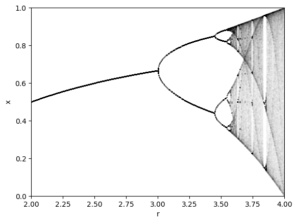
This is better, but the bifurcation points are still blurry because it takes a long time for the system to settle down there. One solution is to increase \(N_0\), but this will increase the computational cost. Another is to use the last iteration \(x\) from the previous \(x\) as \(x_0\) which should put us close to the final attractor. This latter solution works well without increasing the computational cost:
fig, ax = plt.subplots()

N0 = 100
x = x0
rs = np.linspace(r0,r1,Nr)
for r in rs:
    # x = x0   # Use the previous value of x
    for n in range(N0):
        x = f(x, r=r)
    xs = []
    for n in range(N):
        x = f(x, r=r)
        xs.append(x)
    ax.plot([r]*len(xs), xs, '.', ms=0.1, c='k')
ax.set(xlabel='$r$', ylabel='$x$');
There are further refinements one could make: for example, when the system converges quickly to a low period cycle, we still perform \(N\) iterations and plot \(N\) points. One could implement a system that checks to see if the system has converged, then finds the period of the cycle so that only these points are plotted. Such a system should fall back to the previous method only when the period becomes too large. Another sophisticated approach would be to track the curves on the bifurcation plot and plot these as smooth curves. These require some book keeping and we keep our current algorithm which we now code as a function. A final modification we add is allowing the points to be transparent which enables us to see the relative density of points.
def bifurcation(r0=2, r1=4, Nr=500, x0=0.2, N0=500, N=2000, alpha=0.1,
                rs_xs=None):
    """Draw a bifurcation diagram"""
    if rs_xs is not None:
        rs, xs = rs_xs
    else:
        rs = np.linspace(r0,r1,Nr)
        xs = []
        x = x0
        for r in rs:
            for n in range(N0):
                x = f(x, r=r)
            _xs = [x]
            for n in range(N):
                _xs.append(f(_xs[-1], r=r))
            xs.append(_xs)
    _rs = []
    _xs = []
    for r, x in zip(rs, xs):
        _rs.append([r]*len(x))
        _xs.append(x)
    plt.plot(_rs, _xs, '.', ms=0.1, c='k', alpha=alpha)
    plt.axis([r0, r1, 0, 1])
    plt.xlabel('r')
    plt.ylabel('x')

    return rs, xs

rs_xs = bifurcation()
Fixed Points#
The fixed points can be easily deduced by finding the roots of \( x = f^{(n)}(x)\) where the power here means iteration \(f^{(2)}(x) = f(f(x))\)
Show code cell content
import sympy
sympy.init_printing()
x, r = sympy.var('x, r')

def fn(n, x=x):
    for _n in range(n):
        x = f(x, r)
    return x
Period 1#
Here are the period 1 fixed points. The solution at \(x=0\) is trivial, but there is a nontrivial solution \(x = 1 - r^{-1}\) if \(r\geq 1\):
Show code cell content
r1s = sympy.solve(fn(1) - x, r)
r1 = sympy.lambdify([x], r1s[0], 'numpy')  # Makes the solution a function
r1s

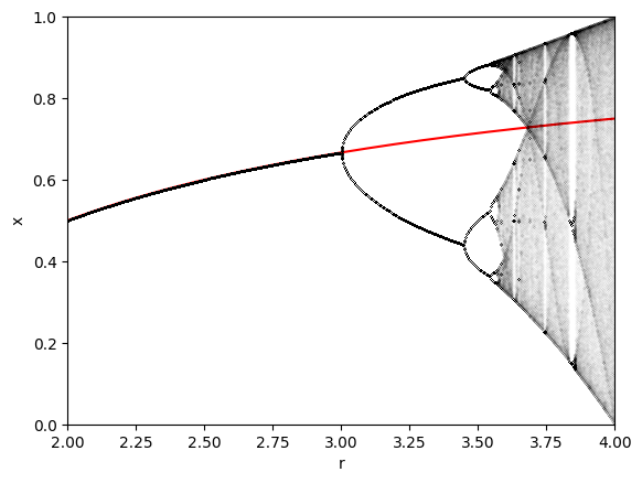
Show code cell source
xs = np.linspace(0, 1.0, 100)[1:-1]
plt.plot(r1(xs), xs, 'r')
bifurcation(rs_xs=rs_xs);
Period 2#
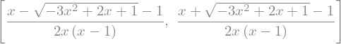
For period 2 we have the solutions for the period 1 equations since these also have period 2, and two new solutions of which only one is positive:
Show code cell content
r2s = sympy.solve((fn(2) - x)/(r-r1s[0])/x/(x-1), r)
r2 = sympy.lambdify([x], r2s[0], 'numpy')
r2s
Show code cell source
xs = np.linspace(0, 1.0, 100)[1:-1]
plt.plot(r1(xs), xs, 'r')
plt.plot(r2(xs), xs, 'g')
bifurcation(rs_xs=rs_xs);
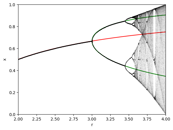
Period 3 Implies Chaos#
In 1975, Li and Yorke proved that Period 3 Implies Chaos in 1D systems by showing that if there exists cycles with period 3, then there are cycles of all orders. Here we demonstrate the period 3 solution.
Show code cell source
res = sympy.factor((fn(3) - x)/x/(r-r1s[0])/(x-1))

coeffs = sympy.lambdify([r], sympy.Poly(res, x).coeffs(), 'numpy')

def get_x3(r, _coeffs=coeffs):
    return sorted([_r for _r in np.roots(coeffs(r)) if np.isreal(_r)])


xs = np.linspace(0, 1, 100)[1:-1]
plt.plot(r1(xs), xs, 'r')
plt.plot(r2(xs), xs, 'g')

r0 = 1+np.sqrt(8)
rs = np.linspace(r0+1e-12, 4, 100)
xs = np.array(list(map(get_x3, rs)))
plt.plot(rs, xs, 'b');
bifurcation(rs_xs=rs_xs);
Exact solution for \(r=4\): Angle doubling on the unit circle#
The chaos at \(r=4\): \(x\mapsto 4x(1-x)\) is special in that the evolution admits an exact solution by transforming to a new variable \(\theta\):
From the identity:
Thus, letting \(x_n = \sin^2\theta_n\) and \(x_{n+1} = \sin^2\theta_{n+1}\) we now have the almost trivial map \(\theta \mapsto 2\theta\), which has the explicit solution \(\theta_n = 2^n\theta_0\). Hence the logistic map with \(r=4\) has the solution:
This evolution is equivalent to moving arround a unit circle by doubling the angle at each step. If \(\theta_0\) is a rational fraction of \(2\pi\) then the motion will ultimately become periodic, but if \(\theta_0\) is an irrational factor of \(2\pi\), then the motion will never be periodic.
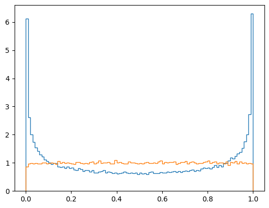
Pseudo-Random Numbers#
This chaotic map may be used as a way of generating pseudo-random numbers from a given seed \(\theta_0 = 2\pi y_0\) where we should ensure that \(y_0\) is irrational.
x0 = np.sqrt(2) % 1
N = 99999
x = [x0]
for n in range(1, N):
    x.append(4*x[-1]*(1-x[-1]))
x = np.array(x)
y = np.arcsin(np.sqrt(x))*2/np.pi
args = dict(bins=100, density=True, histtype='step')
plt.hist(x, **args);
plt.hist(y, **args);
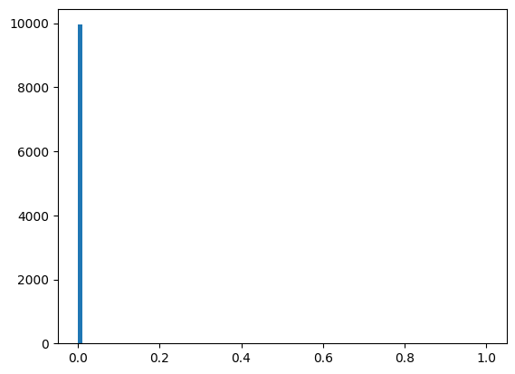
y0 = np.sqrt(2) % 1
N = 10000
y = [y0]
for n in range(1, N):
    y.append(1 - abs(2*y[-1] - 1))
y = np.array(y)
x = np.sin(2*np.pi * y)**2
plt.hist(x, bins=100);
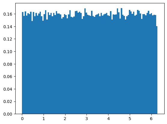
y0 = np.sqrt(2) % 1
th0 = 2*np.pi * y0
N = 100000
th = [th0]
for n in range(1, N):
    th.append((2*th[-1]) % (2*np.pi))
th = np.array(th)
x = np.sin(th)**2
plt.hist(th, bins=100, density=True);
Feigenbaum Constants (Incomplete)#
First we define some notation. Let \(r_{n}\) be the smallest value of the growth parameter where the period bifurcates from \(2^{n-1}\) to \(2^{n}\). Define the iterated function as:
The first bifurcation point is at \(r_{1} = 3\), \(x_{1} = 2/3\), i.e. the solution to \(x_1 = f_{r_1}(x_1)\). At this point, the fixed point becomes unstable: \(\abs{f'_{r_{1}}(x_{1})} = 1\). Now, since \(x_{1}\) is a fixed point of \(f_{r_1}(x)\), it must also be a fixed point of \(f^{(2)}_{r_1}(x)\). We plot both of these below, as well as \(f^{(2)}_{r_1+\epsilon}(x)\) for a slightly larger \(r = r_1 + \epsilon\):
Show code cell source
x = np.linspace(0, 1)
r_1 = 3.0
epsilon = 0.2
r_1a = r_1 + epsilon

fig, ax = plt.subplots()
ax.plot(x, x, 'k')
ax.plot(x, f(x, r=r_1), 'C0', label="$f_{r_1}(x)$")
ax.plot(x, f(f(x, r=r_1), r=r_1), 'C1', label="$f^{(2)}_{r_1}(x)$")
ax.plot(x, f(f(x, r=r_1a), r=r_1a), 'C1', ls='--', label=f"$f^{{(2)}}_{{r_1+{epsilon:.1f}}}(x)$")
ax.legend()
ax.set(xlabel="$x$", title=f"$r_1={r_1}$");
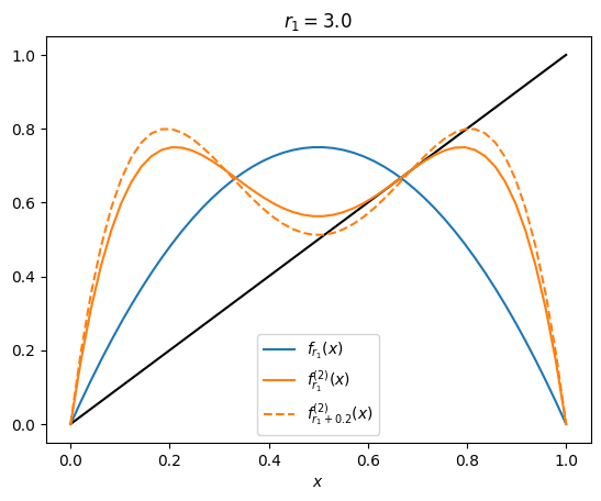
Notice the behaviour that, at this shared fixed point, \(f^{(2)}_{r_1}{}'(x) = \bigl(f'_{r_1}(x)\bigr)^2 = 1\). As we increase \(r = r_1+\epsilon\), this steepens and the two new fixed points move outward.
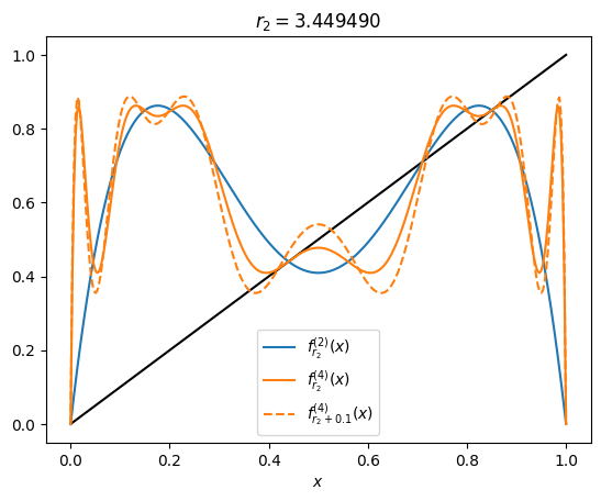
We now look at \(f^{(2)}_{r_2}(x)\) and \(f^{(4)}_{r_2}(x)\), where we see the same behaviour about both of the new fixed points:
Show code cell source
x = np.linspace(0, 1, 300)
r_2 = 1+np.sqrt(6)
def f2(x, r=r_2):
    return f(f(x, r), r)
epsilon = 0.1
r_2a = r_2 + epsilon

fig, ax = plt.subplots()
ax.plot(x, x, 'k')
ax.plot(x, f2(x), 'C0', label="$f^{(2)}_{r_2}(x)$")
ax.plot(x, f2(f2(x)), 'C1', label="$f^{(4)}_{r_2}(x)$")
ax.plot(x, f2(f2(x, r=r_2a), r=r_2a), 'C1', ls='--', label=f"$f^{{(4)}}_{{r_2+{epsilon:.1f}}}(x)$")
ax.legend()
ax.set(xlabel="$x$", title=f"$r_2={r_2:.6f}$");
Show code cell source
x = np.linspace(0, 1, 10000)
rr = 3.5699456718709449018420051513864989367638369115148323781079755299213628875001367775263210

def fn(x, n, r=rr):
    for n in range(n):
        x = f(x, r)
    return x

fig, ax = plt.subplots()
ax.plot(x, x, 'k')
for n in range(10):
    ax.plot(x, fn(x, 2**n), 'C1', lw=0.1)
ax.plot(x, fn(x, 1024), 'C0', label="$f^{(1024)}_{r_*}(x)$")
ax.legend()
ax.set(xlabel="$x$", title=f"$r_*={rr:.6f}$");
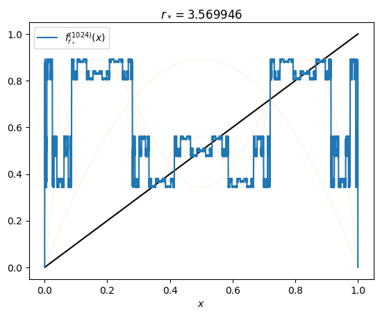
(see Weisstein, Eric W. “Logistic Map”).
\(n\) |
\(r_n\) |
\(\delta_n = \frac{r_{n}-r{n-1}}{r_{n+1}-r{n}}\) |
|---|---|---|
0 |
1 |
|
1 |
3 |
|
2 |
3.449490 |
|
3 |
3.544090 |
|
4 |
3.564407 |
|
5 |
3.568750 |
|
6 |
3.56969 |
rn = np.array([1.0, 3.0,  1+np.sqrt(6),
               3.5440903595519228536, 3.5644072660954325977735575865289824,
               3.568750, 3.56969, 3.56989, 3.569934, 3.569943, 3.5699451,
               3.569945557
               3.5699456718709449018420051513864989367638369115148323781079755299213628875001367775263210342163
               ])