Show code cell content
import mmf_setup; mmf_setup.nbinit()
import os
from pathlib import Path
import logging; logging.getLogger("matplotlib").setLevel(logging.CRITICAL)
%matplotlib inline
import numpy as np, matplotlib.pyplot as plt
This cell adds /home/docs/checkouts/readthedocs.org/user_builds/iscimath-583-fractals/checkouts/latest/src to your path, and contains some definitions for equations and some CSS for styling the notebook. If things look a bit strange, please try the following:
- Choose "Trust Notebook" from the "File" menu.
- Re-execute this cell.
- Reload the notebook.
Solution 1: Darwin and Galton#
Here is a partial solution to Assignment 1: Darwin and Galton. Try it first!
The Gambler’s Ruin, Random Walks, and Information Theory#
from uncertainties import ufloat

rng = np.random.default_rng(seed=2024)

def play(p=0.5, K=0, B=100):
    n_plays = 0
    while K > 0 and K < B:
        dK = rng.choice([1, -1], p=[p, 1-p], size=min(K, B-K))
        K += sum(dK)
        n_plays += len(dK)
    ruin = K <= 0

    return ruin

K = 10
B = 11
q = [play(K=K, B=B) for n in range(10000)]
q_k = ufloat(np.mean(q), np.std(q)/np.sqrt(len(q)))
print(f"{q_k=:S}, {1-K/B=:.2g}")
q_k=0.0894(29), 1-K/B=0.091
More Food for Fair Thought#
One way of testing the reliability of Galton’s rank-order statistic \(N\) – the number of rank-order pairs in which the crossed heights exceed the self-fertilized heights – is to make a definite model and simulate the results. The code in Assignment 1: Darwin and Galton suggests that if the plant heights are distributed uniformly, then each outcome \(N \in \{0, 1, 2, \dots, 15\}\) is equally likely. This supports Schroeder’s claim ([Schroeder, 1991]) that, even with absolutely no differences, \(3/16\) of the time, Galton’s method would have found a compelling difference!
One potential flaw is the assumption that the plant-heights are uniformly distributed. One can perform the analysis with different distributions to become more confident.
This leads to the question – given some samples (data) \(D=\{h_1, h_2, \dots, h_N\}\), how consistent are these with a given distribution (PDF) \(p(h)\)? This is not a straightforward problem, but strategies exist, including applying the Kolmogorov-Smirnov test. To better understand, one can easily form the probability (or likelihood) that the data came from a given distribution:
This can be combined with Bayes’ theorem to give a probability that \(p(h)\) is the correct distribution:
The main challenge here is determining an appropriate prior. (A minor challenge is normalizing over the space of distributions.)
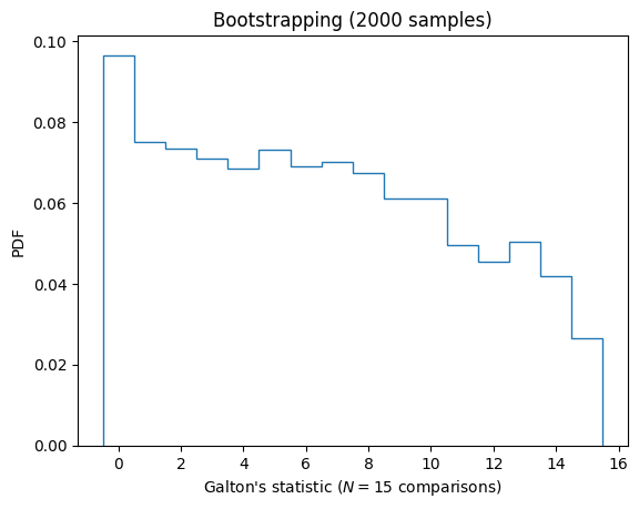
Another strategy is to simply skip over this problem and sample from the original data. This is called bootstrapping. We will not justify it here, but demonstrate that it gives similar results. Here we can test how likely various values of Galton’s rank-order statistic \(N\) are under the assumption that there is no difference between the samples in Darwin’s data:
Show code cell source
height_inches = np.array(
    [[23+4/8, 17+3/8],
     [12, 20+3/8],
     [21, 20],
     [22, 20],
     [19+1/8, 18+3/8],
     [21 + 4/8, 18 + 5/8],
     [22 + 1/8, 18 + 5/8],
     [20 + 3/8, 15 + 2/8],
     [18 + 2/8, 16 + 4/8],
     [21 + 5/8, 18],
     [23 + 2/8, 16 + 2/8],
     [21, 18],
     [22 + 1/8, 12 + 6/8],
     [23, 15 + 4/8],
     [12, 18]])

def galton(h):
    """Return the number of cases where the first rank-orderd column is bigger."""
    inds = np.argsort(h, axis=0)
    sorted_h = np.concatenate([[h[i]] for i, h in zip(inds.T, h.T)]).T
    assert np.all(np.diff(sorted_h, axis=0) >= 0)
    N = (np.diff(sorted_h, axis=1) > 0).sum()
    return N

rng = np.random.default_rng(seed=2024)
Nsamples = 2000
N = 15
Ns = [galton(rng.choice(height_inches.ravel(), size=(N, 2))) for n in range(Nsamples)]

fig, ax = plt.subplots()
ax.hist(Ns,
        bins=np.arange(N+2)-0.5, # Make sure our bins are centered
        density=True,            # Normalize to probabilities (PDF)
        histtype='step',         # Don't fill the bars
);
ax.set(title=f"Bootstrapping ({Nsamples} samples)",
       xlabel=f"Galton's statistic (${N=}$ comparisons)",
       ylabel="PDF");
Another related question is – what errors should we plot for these histogram bins?
rng = np.random.default_rng(seed=2024)
Nsamples = 20000
N = 15
Ns = [galton(rng.lognormal(size=(N, 2))) for n in range(Nsamples)]

fig, ax = plt.subplots()
ax.hist(Ns,
        bins=np.arange(N+2)-0.5, # Make sure our bins are centered
        density=True,            # Normalize to probabilities (PDF)
        histtype='step',         # Don't fill the bars
);
ax.set(title=f"Lognormal distribution ({Nsamples} samples)",
       xlabel=f"Galton's statistic (${N=}$ comparisons)",
       ylabel="PDF");

Counterintuition Runs Rampant in Random Runs#
from uncertainties import ufloat

rng = np.random.default_rng(seed=2024)

def duration(p=0.5, K=0, B=100):
    n_plays = 0
    while K > 0 and K < B:
        dK = rng.choice([1, -1], p=[p, 1-p], size=min(K, B-K))
        K += sum(dK)
        n_plays += len(dK)
    ruin = K <= 0

    return n_plays

K = 1
B = 100
D = [duration(K=K, B=B) for n in range(10000)]
D_k = ufloat(np.mean(D), np.std(D)/np.sqrt(len(D)))
print(f"{D_k=:S}, K(B-K)={K*(B-K):.2g}")
D_k=104(6), K(B-K)=99