Fractals#

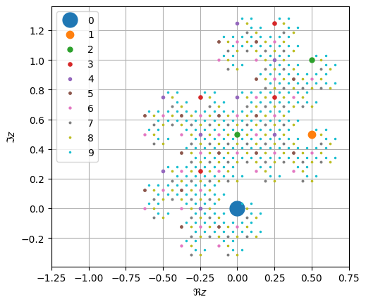
Twindragon#

Here is the construction of the twindragon suggested by expressing all proper binary fractions 0.100101, 0.001101, etc. in base \((1-\I)\). I.e. if \(d_n\) is the \(n\)th digit:

\[\begin{gather*} z = \sum_{n=1}^{\infty} d_n(1-\I)^{-n}\\ z_{0.100101} = \frac{1}{(1-\I)^{1}} + \frac{1}{(1-\I)^{4}} + \frac{1}{(1-\I)^{6}},\\ z_{0.001101} = \frac{1}{(1-\I)^{3}} + \frac{1}{(1-\I)^{4}} + \frac{1}{(1-\I)^{6}},\\ z_{0.\bar{1}} = \frac{1}{(1-\I)^{1}} + \frac{1}{(1-\I)^{2}} + \cdots = \I. \end{gather*}\]

Noting that \(1-\I = \sqrt{2}e^{-\pi \I/4}\), we have

\[\begin{gather*} \left\lvert\frac{1}{(1-\I)^n}\right\rvert = \frac{1}{\sqrt{2}^n}. \end{gather*}\]

base = (1-1j)

q = 1/base
points = np.array([0])
N = 10

fig, ax = plt.subplots()
ms0 = 30
collection = list(ax.plot(points.real, points.imag, '.', ms=ms0, label="0"))
labels = ["0"]

for n in range(1, N):
    new_points = points + q
    collection.append(
        ax.plot(new_points.real, new_points.imag, '.', ms=ms0/(1+n), label=str(n)))
    labels.extend(str(n))
    points = np.concatenate([points, new_points])
    q /= base
ax.set(xlim=(-1.25,0.75), aspect=1, xlabel=r"$\Re z$", ylabel=r"$\Im z$")
ax.grid(True)
plt.legend();

#from mpld3 import plugins
#interactive_legend = plugins.InteractiveLegendPlugin(collection, labels)
#plugins.connect(fig, interactive_legend)
#mpld3.display()

../_images/5a72a0dc0bf7ee866e8fb4a88ee385f5997e2767fa471fbf6a9200b53d799fb3.png

base = (1-1j)

q = 1/base
points = np.array([0])
strings = np.array(['0.'])

N = 11

for n in range(1, N):
    new_points = points + q
    points = np.concatenate([points, new_points])
    strings = np.concatenate([np.char.add(strings, '0'), np.char.add(strings, '1')])
    q /= base

fig, ax = plt.subplots()
collection, = ax.plot(points.real, points.imag, '.')
ax.set(xlim=(-1.25,0.75), aspect=1, xlabel=r"$\Re z$", ylabel=r"$\Im z$")
ax.grid(True)

import mpld3
mpld3.plugins.connect(fig, mpld3.plugins.PointLabelTooltip(collection,
                      labels=strings.tolist(), location="bottom right"))
mpld3.display()

---------------------------------------------------------------------------
ModuleNotFoundError                       Traceback (most recent call last)
Cell In[3], line 20
     17 ax.set(xlim=(-1.25,0.75), aspect=1, xlabel=r"$\Re z$", ylabel=r"$\Im z$")
     18 ax.grid(True)
---> 20 import mpld3
     21 mpld3.plugins.connect(fig, mpld3.plugins.PointLabelTooltip(collection,
     22                       labels=strings.tolist(), location="bottom right"))
     23 mpld3.display()

ModuleNotFoundError: No module named 'mpld3'

../_images/f64e9f057fa1aa1e4df58b88ce5b2996fecd81f759ba8ede9d0097323d9d6d84.png

What numbers lie on the boundaries?

The boundary points can be generated from the strings of digits accepted by a 6-state automaton.

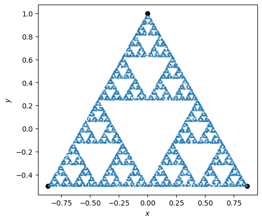
Sir Pinski’s Game and Deterministic Chaos#

Chapter 1: [Schroeder, 1991].

Here we play Sir Pinski’s game.

Note

To simplify the implementation, we use complex numbers \(z=x+\I y\) to represent the points. This makes it easy, for example, to define the vertices \(p_n\) of an equilateral triangle:

\[\begin{gather*} p_n = r e^{2\pi \I n / 3} e^{\I \pi/2}. \end{gather*}\]

To plot these, we need a function z2xy() that extracts and packages the real and imaginary parts into an appropriate array so that they can be plotted. We use a property of NumPy arrays that allows a complex array to be viewed as a real array with twice as many elements. We then reshape things so that the first index selects \(x\) and \(y\).

We now iterate as follows:

\[\begin{gather*} z_{n+1} = \frac{z_{n} + p_{n}}{2}\\ z_{1} = \frac{z_0}{2} + \frac{p_0}{2}\\ z_{2} = \frac{z_0}{2^{2}} + \frac{p_1}{2} + \frac{p_0}{2^2}\\ z_{3} = \frac{z_0}{2^{3}} + \frac{p_2}{2} + \frac{p_1}{2^{2}} + \frac{p_0}{2^{3}}\\ \vdots\\ z_{n} = \frac{z_0}{2^{n}} + \sum_{j=0}^{n-1}\frac{p_j}{2^{n-j}} = \frac{z_0}{2^{n}} + \frac{1}{2^{n}}\sum_{j=0}^{n-1} 2^{j}p_j. \end{gather*}\]

where \(p_{n}\) is one of the vertices, randomly chosen.

../_images/2604a4fd4be9a5d9b7a719ff8f8fad8cba2df82a021aae2e4dbb755de37582f8.png

Fractals

Contents

Fractals#

Twindragon#

Sir Pinski’s Game and Deterministic Chaos#