Solution 9: Newton’s Method#

Here is one way to try to find an attractive cycle. Let’s start with the original cubic polynomial \(g(z) = z^3 - 1\) and move the root at \(r_1 = 1\) to a new root at \(c\), which will be our “parameter”:

\[\begin{gather*} g(z) = \frac{(z^3 - 1)(z-c)}{z-1} = \underbrace{(z^2 + z + 1)}_{(z-q)(z-\bar{q})}(z-c),\\ g'(z) = 3z^2 + (2z + 1)(1-c), \\ g''(z) = 6z + 2(1-c) = 6\Bigl(z - \underbrace{\frac{c-1}{3}}_{z_0}\Bigr). \end{gather*}\]

Our Newton iteration is

\[\begin{gather*} f(z) = \frac{2z^3 + z^2(1-c) + c} {3z^2 + (2z + 1)(1-c)},\qquad z_0 = \frac{q + q^* + c}{3} = \frac{c-1}{3},\\ f'(z) = \frac{\overbrace{(z^2 + z + 1)(z - c)}^{g(z)}\overbrace{2(3z + 1 - c)}^{g''(z)}} {(3z^2 + (2z+1)(1-c))^2} \end{gather*}\]

We first simply start from \(z_0\) and iterate a bunch of times, plotting the final point. If this state is attracted to one of the roots, then after a large number of iterations, \(g(z_n) \approx 0\). But if \(z_0\) is attracted to a periodic cycle, \(z_n\) will not be a root, and so we should see some deviations:

../_images/d73913036b2b30fa4cbfb604d9ff674253e506f82a2453fe493d2eb7091b6a17.png

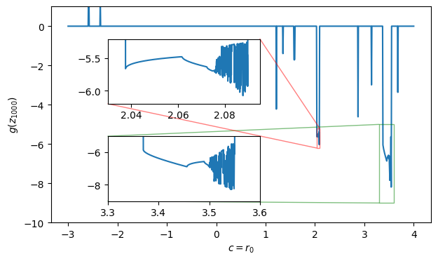
We see that there are several places where we appear to have an attractive cycle. We have zoomed in on two such places near \(r_0=2.06\) and \(r_0=3.5\). If you look carefully at these insets, you might notice that it appears we are tracing part of some Bifurcation Diagrams. This is a pretty good hint that there is a Mandelbrot-like set hidden somewhere nearby.

Here we try to find it

Show code cell source Hide code cell source

%matplotlib inline
import numpy as np, matplotlib.pyplot as plt
import numba

# Since we want to pass in the roots as an array, we must generalize and use
# guvectorize, which means we must write our own loop.  Note also that even scalar
# arguments must be arrays
@numba.guvectorize(
    ["(complex128[:,:], complex128[:], float64[:], int_[:], int32[:,:])"],
    "(m,n),(i),(),()->(m,n)",
    cache=True,
    target="parallel",
)
def _convergence_time(c, roots, eps, maxiter, n):
    for x in range(c.shape[0]):
        for y in range(c.shape[1]):
            roots[0] = c[x, y]
            z = roots.mean()
            for n[x, y] in range(maxiter[0] + 1):
                g = 1 + 0j
                tmp = 0j
                for r_i in roots:
                    g *= (z-r_i)
                    tmp += 1/(z-r_i)
                z -= 1/tmp
                if g.real**2 + g.imag**2 <= eps[0]:
                    break

def convergence_time(c, roots, eps=1e-8, maxiter=100):
    """Return the "convergence time" of initial point `z0` under Newton's method.

    Arguments
    ---------
    c : complex
        Location in the Mandelbrot set.
    roots : complex array
        Roots of the polynomial.
    eps : float
        Bailout radius.
    maxiter : int
        Maximum number of iteration.  If the iteration does not terminate before this,
        then this value is returned.  It can be used as an approximation of the interior
        of the sets.
    """
    return _convergence_time(c, roots, eps, maxiter)


# Try changing the ranges here
N = 256

roots = np.exp(2j*np.pi * (np.arange(3)/3.0))
c, R = 1.578 + 0j, 0.01
c, R = 1.1395 + 0j, 0.001
c, R = 3.4 + 0j, 0.2

x = np.linspace(c.real - R, c.real + R, N)
y = np.linspace(c.imag - R, c.imag + R, N)
z = x[:, None] + 1j*y[None, :]

# Try changing maxiter - especially if you get deep.
%time n = convergence_time(z, roots, maxiter=1000)

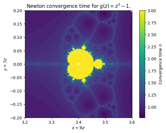
fig, ax = plt.subplots()
mesh = ax.pcolormesh(x, y, np.log10(n).T, shading='auto')
ax.plot(roots.real, roots.imag, 'ow')
ax.plot([c.real], [c.imag], 'xw')

fig.colorbar(mesh, label=r"Convergence time $n$")
ax.set(xlabel=r"$x = \Re z$", ylabel=r"$y = \Im z$", 
       xlim=(x.min(), x.max()), ylim=(y.min(), y.max()),
       title=f"Newton convergence time for $g(z)=z^3-1$.",  aspect=1);

CPU times: user 217 ms, sys: 596 µs, total: 218 ms
Wall time: 203 ms

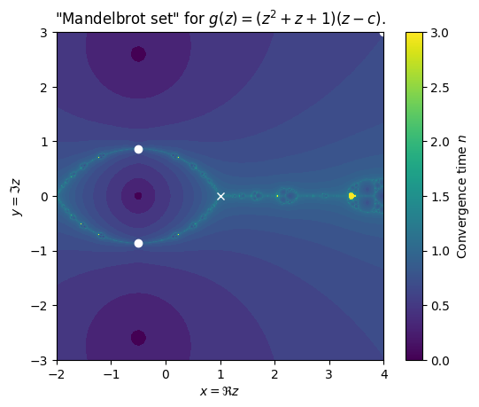
../_images/769161c5461999fa96ed3ba3f52b9f733d436642202433e7138dc6d565b0e91f.png

Here we zoom out. Note: this is a rotated and scaled version of the set shown in the 3Blue1Brown video. They look at the region on the left side of this figure.

CPU times: user 269 ms, sys: 0 ns, total: 269 ms
Wall time: 255 ms

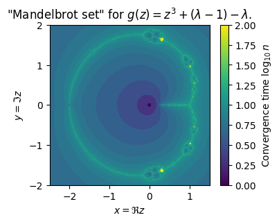
../_images/3912aa434bc9fbfed4966a4796eb45ba389f0e80ff910ede61ce715d125841bd.png

Alternative Approach#

The qualitative picture will not change if we perform an affine transformation of the plane. I.e rotations, translations, and scalings. Thus, given an arbitrary cubic polynomial, we can always translate, rotate, and scale so that the mean of the roots \(z_0 = 0\) lies at the origin, and so that one of the roots lies at \(r_0 = 1\). The two other roots must satisfy \(r_1 + r_2 = -1\). Thus, we have

\[\begin{gather*} g(z) = (z-1)(z-r_1)(z-r_2) = z^3 - \underbrace{(1+r_1+r_2)}_{0}z^2 + (\underbrace{r_1r_2}_{\lambda} + \underbrace{r_1 + r_2}_{-1})z - \underbrace{r_1r_2}_{\lambda}\\ = z^3 + (\lambda - 1)z - \lambda,\\ g'(z) = 3z^2 + \lambda - 1, \qquad g''(z) = 6z,\qquad f(z) = \frac{2z^3 + \lambda}{3z^2 + \lambda - 1}. \end{gather*}\]

CPU times: user 2.37 s, sys: 3.56 ms, total: 2.38 s
Wall time: 1.25 s

../_images/d2acd58bdce21362647b8c27064a860356db3ed5ea016fca7b51f311c2973435.png

../_images/8aae9bd150a52e1c302518dc3ecebd4b7a9931c3c1c059ab02cfb93cce526738.png

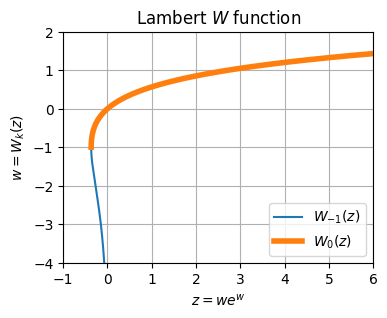
Lambert \(W\) Function#

Here we explore trying to find a globally convergent method for computing the Lambert \(W_0(z)\):

\[\begin{gather*} z = we^w, \qquad W_0(z) = w, \qquad z\geq -\frac{1}{e}, \qquad w\geq -1. \end{gather*}\]

Let’s start with the following Newton iteration

\[\begin{gather*} g_z(w) = we^{w} - z, \qquad g_z'(w) = (1+w)e^{w}, \\ w\mapsto f_z(w) = w - \frac{g_z(w)}{g_z'(w)} = \frac{w^2 + ze^{-w}}{1+w}. \end{gather*}\]

../_images/e4c42d62ae9b10542ef66e04c97ec97d96549faac8d7084dbb3b03636e14cb79.png

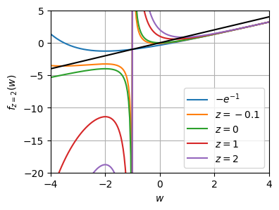
We show what \(w \mapsto f_z(w)\) looks like on the right. Due to the pole at \(w=-1\), we expect that we must start with \(w_0 \geq -1\) if we want to converge to the \(k=0\) branch.

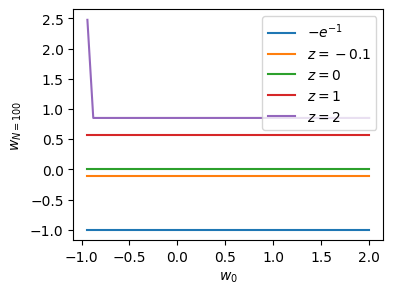
Now lets see what the region of convergence is for \(z = 1\) (lower figure on the right). Modulo some floating point issues close to \(w_0=-1\) (where the denominator vanishes) and \(z=-e^{-1}\) (where we rely on a subtle cancellation to get \(w=-1\)), we see that all initial guesses converge to the desired root.

/tmp/ipykernel_4253/164599588.py:8: RuntimeWarning: divide by zero encountered in divide
  return (w**2 + z*np.exp(-w))/(1+w)
/tmp/ipykernel_4253/164599588.py:8: RuntimeWarning: invalid value encountered in divide
  return (w**2 + z*np.exp(-w))/(1+w)

../_images/34b05a9ca47f6b3e58f689441d1ce15aa287e9df084ee37b737facb2c5abc732.png

We will need to tidy up the region near \(w=-1\), but away from this, we can now see how long it takes for Newton’s method to converge to a desired accuracy.

@numba.vectorize("int32(float64, float64, int_, float_)", cache=True, target="parallel")
def _escape_time(z, w, maxiter, eps):
    for n in range(maxiter):
        w = (w**2 + z*np.exp(-w))/(1+w)
        g = w*np.exp(w) - z
        if abs(g) < eps:
            break
    return n

def escape_time(z, w0, maxiter=100, eps=1e-12):
    return _escape_time(z, w0, maxiter, eps)
    
z = np.linspace(-np.exp(-1), 3)[1:]
w0 = np.linspace(-1, 2, 101)[1:]

n = escape_time(z[:, None], w0[None, :], 10)

fig, ax = plt.subplots()
mesh = ax.pcolormesh(z, w0, n.T)
ax.set(xlabel="$z$", ylabel="$w_{0}$");
fig.colorbar(mesh, label=r"Convergence time $n$");

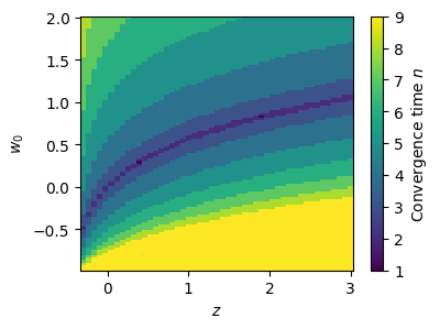
../_images/5ba633e6da751297fd4b8f0594cefaf8945351225825e7571c38424c61f37dd1.png

We see that if we can get close-enough to the solution for an initial guess, then we can converge in a few iterations. Thus an initial guess of \(w_0 = 1\) will probably work quite well for \(z\in [0, 5]\). For larger and smaller \(z\) we will need to do something else.

How to proceed? One can try to make series approximations or look at the asymptotic behavior of the function to get an initial guess. For example, we might expand about \(w = -1 + \epsilon\):

\[\begin{gather*} z = (\epsilon -1)e^{\epsilon - 1} = \frac{\epsilon - 1}{e}\left(1 + \epsilon + \frac{\epsilon^2}{2} + \cdots\right). \end{gather*}\]

Keeping terms to quadratic order, we have

\[\begin{gather*} z \approx \frac{\epsilon^2 - 1}{e}, \qquad \epsilon \approx \sqrt{1 + ez}, \qquad w \approx \sqrt{1 + ez} - 1. \end{gather*}\]

Let’s see how well using \(w_0 = \sqrt{1 + e z} - 1\) converges.

@np.vectorize
def nW1(z, maxiter=12, eps=1e-12):
    w = np.sqrt(1 + np.exp(1)*z) - 1
    for n in range(maxiter):
        w = (w**2 + z*np.exp(-w))/(1+w)
        g = w*np.exp(w) - z
        if abs(g) < eps:
            break
    return n

@np.vectorize
def nW2(z, maxiter=12, eps=1e-12):
    w = 1
    for n in range(maxiter):
        w = (w**2 + z*np.exp(-w))/(1+w)
        g = w*np.exp(w) - z
        if abs(g) < eps:
            break
    return n

z = np.linspace(-np.exp(-1), 5, 1000)[1:]

fig, ax = plt.subplots()
ax.plot(z, nW1(z), label=r"$w_0 = \sqrt{1+ez}-1$")
ax.plot(z, nW2(z), label=r"$w_0 = 1$")
ax.legend()
ax.set(xlabel="$z$", ylabel="convergence time $n$");

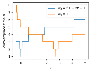
../_images/5775ed2c46ffde96da5bde0effb285ce8ab1f972977b0778c03f15cc7f04cf39.png

This tells us that a reasonable strategy might be to switch guesses at \(z=1\). We still have an issue for larger \(z\). Some ideas for improving this.

Asymptotic expansions. Try a series expansion in \(1/z\) or \(1/w\). Unfortunately, in this case, the asymptotic behaviour is defined by the Lambert function, which is one of the reasons it is useful to have a solution. So this does not help here.
Choose different \(w_0\) for larger \(z\). Perhaps one can guess a reasonable form? This is likely not going to help for very large \(z\), but might get a practical solution if you know you will only need solutions for e.g. \(z<100\).
We directly applied Newton’s method to \(g(z) = we^w - z\), but it can be applied to many different forms of this equation. Some of these might converge better for large \(z\). For example:

\[\begin{gather*} g(w) = e^w - z/w,\\ g(w) = w + \ln w - \ln z,\\ \dots. \end{gather*}\]

Solution 9: Newton’s Method

Contents

Solution 9: Newton’s Method#

Alternative Approach#

Lambert \(W\) Function#

References#