Julia Sets#

There are several ways of defining Julia sets. We start with the discussion in [Falconer, 2014] by introducing a holomorphic function \(f: \mathbb{C} \mapsto \mathbb{C}\) that is generally considered to be a polynomial \(f(z) = p(z)\), but, as Falconer mentions, many results extend to rational functions \(f(z) = p(z)/q(z)\) or meromorphic function.

[Falconer, 2014] defines the Julia set \(J(f)\) as the boundary of the filled-in Julia set \(K(f)\):

\[\begin{gather*} K(f) = \{z \in \mathbb{C} \mid \lim_{k\rightarrow \infty} f^{(k)}(z) = f(f(f(\cdots f(z)\cdots ))) \neq \infty \}, \\ J(f) = \partial K(f). \end{gather*}\]

Some related properties from [Falconer, 2014] for polynomial \(f(z)\):

Lemma 14.1: There is some radius \(r\) such that if \(\abs{f^{k}(z)} > r\), then \(f^{k}(z) \rightarrow \infty\). Thus, it suffices to see if an initial point ever exceeds this bailout radius \(r\).
Proposition 14.3: The Julia set is forward and backward invariant under \(f\):

\[\begin{gather*} J = f(J) = f^{-1}(J). \end{gather*}\]
Theorem 14.10: \(J(f)\) is the closure of the set of repelling periodic points of \(f\).

Lemma 14.11: If \(w\) is an attractive fixed point of \(f\), then \(J(f) = \partial A(w)\) where \(A(w)\) is the basin of attraction of \(w\):

\[\begin{gather*} A(w) = \{z\in \mathbb{C} \mid \lim_{k\rightarrow \infty} f^{k}(z) \rightarrow w\}. \end{gather*}\]

This also applies for \(w=\infty\), which we use below in the BSM method.

Since we are focusing on holomorphic functions, it is easy to determine whether or not a fixed-point is attractive or repulsive: one simply computes the absolute value of the derivative:

Attractive: \(\abs{f'(z)} < 1\),
Indiferent: \(\abs{f'(z)} = 1\),
Repulsive: \(\abs{f'(z)} > 1\).

Several algorithms can be used to draw/sample Julia sets, many of which are discussed in [Barnsley et al., 1988]. We now discuss and implement some of these so that you can use them as sources for testing your dimension extraction code. We specialize here to the usual quadratic case

\[\begin{gather*} f_c(z) = z^2 + c \end{gather*}\]

but generalizing to other functions is almost trivial. In this case, the fixed points of the Julia set \(J_c\) have the following form:

\[\begin{gather*} z = f_c(z) = z^2 + c, \\ z_{\pm} = \frac{1 \pm \sqrt{1 - 4c}}{2},\\ \abs{f'(z_\pm)} = 2\abs{z_{\pm}} = \abs{1 \pm \sqrt{1 - 4c}}. \end{gather*}\]

Several of the algorithms discussed below have difficulty near indifferent fixed points.

Do it! Find the set of \(c_1\) where \(J_c\) has indifferent fixed points.

We are looking for the set of \(c\) which satisfy

\[\begin{gather*} 1 = (1 \pm \sqrt{1 - 4c})(1 \pm \sqrt{1 - 4c}^*) = 1 \pm 2\Re\sqrt{1 - 4c} + \abs{1 - 4c}. \end{gather*}\]

Let \(q = \sqrt{1 - 4c} = x + \I y\), then the set of \(c\) where one of the fixed points of \(J_c\) is indifferent can be expressed in terms

\[\begin{gather*} y = \pm \sqrt{2\abs{x} - x^2}, \qquad x \in [-2, 2],\\ q = x+ \I y = x \pm \I \sqrt{2\abs{x} - x^2},\\ c = \frac{1-q^2}{4} = \frac{1 + 2x(1-x) \pm 2\I \sqrt{x^3(1-2x)}}{4}. \end{gather*}\]

With some algebra, one can derive an alternative parameterization proceeding as follows. The condition for a fixed-point and indifference are

\[\begin{gather*} z = f^{(1)}(z) = z^2 + c, \qquad \abs{f^{(1)}_{,z}} = \abs{2z} = 1. \end{gather*}\]

Hence, we let \(q = f^{(1)}_{,z} = 2z = e^{\I\theta}\). Solving for \(c\) we have

\[\begin{gather*} c = z - z^2 = \frac{q(2-q)}{4}. \end{gather*}\]

Thus:

\[\begin{gather*} c_1 = \frac{e^{\I\theta}(2 - e^{\I\theta})}{4}, \qquad \theta = 2\pi t \in [0, 2\pi], \qquad t \in [0, 1]. \end{gather*}\]

This is the boundary of the main cardioid of the Mandelbrot set \(M\). The “bulbs” occur for rational \(t\).

Do it! Find the set \(c_2\) where \(J_c\) has indifferent period-2 attractors.

We are now looking for the set of \(c\) which satisfy

\[\begin{gather*} z = f^{(2)}(z) = (z^2+c)^2 + c, \qquad \abs{f^{(2)}_{,z}(z)} = \abs{4z(z^2 + c)} = 1. \end{gather*}\]

Again, we set \(q = 4z(z^2 + c) = e^{\I\theta}\). This should include the period-1 fixed-point \(c_1 = z-z^2\), so we expect the first equation to factor, and indeed, it does:

\[\begin{gather*} (z^2+c)^2 + c - z = (c - z + z^2)(c + 1 + z + z^2) = 0. \end{gather*}\]

The period two solution must be the second root:

\[\begin{gather*} c_2 = -1 - z - z^2. \end{gather*}\]

Inserting this into the equation for \(q\), we have

\[\begin{gather*} q = -4z(1+z), \qquad z + z^2 = \frac{-q}{4}. \end{gather*}\]

Combining these gives \(c_2 = q/4 - 1\):

\[\begin{gather*} c_2 = \frac{e^{\I\theta}}{4} - 1, \qquad \theta \in [0, 2\pi]. \end{gather*}\]

Do it! Repeat for period-3 attractors. (Hard, incomplete.)

We are now looking for the set of \(c\) which satisfy

\[\begin{gather*} z = f^{(3)}(z) = \Bigl((z^2+c)^2 + c\Bigr)^2 + c, \qquad \abs{f^{(3)}_{,z}(z)} = \abs{8z(z^2 + c)((z^2 + c)^2 + c)} = 1. \end{gather*}\]

First set \(f^{(3)}_{,z}(z) = q = e^{\I\theta}\). As before, we expect the first equation to have a factor of \(z^2+c - z\) since period-1 fixed-points are also period 3 fixed points. This leaves a cubic equation for \(c_3\), and the full solution can be expressed as:

\[\begin{align*} P(z, c) &= c^3 + (3z^2 + z + 2)c^2 + (3z^4 + 2z^3 + 3z^2 + 2z + 1)c + z^6 + z^5 + z^4 + z^3 + z^2 + z^1 + z^0 = 0,\\ Q(z, c) &= 8z(z^2 + c)\Bigl((z^2 + c)^2 + c\Bigr) - q = 0. \end{align*}\]

(In the notation of [Giarrusso and Fisher, 1995], the first expression is \(F_{3}(z)\) and \(\lambda = 2^{-3}q\) with \(q=\rho\).) We are thus looking for the simultaneous solution of two polynomial equations:

\[\begin{gather*} P(z, c) = 0, \qquad Q(z, c) = 0. \end{gather*}\]

In principle, we can solve these, but one will have to deal with what [Giarrusso and Fisher, 1995] calls branching problems, when instead, we want a closed form solution \(c(q)\). This can be done as shown in [Giarrusso and Fisher, 1995] but is not trivial.

Boundary Scanning Method (BSM)#

This method works when \(c\) is well within the Mandelbrot set so there is an interior – we look at each box, and if some points are inside in \(K_c\) while others are outside in \(A_c(\infty)\), we declare that box to contain an element of \(J_c\). This approach will not work for \(c\notin M\) where \(J_c\) has measure zero.

This uses the following notions from [Barnsley et al., 1988], making use of Lemma 14.1, Proposition 14.3, and Lemma 14.11:

\[\begin{gather*} A_c(\infty) = \{z_0 \in \mathbb{C} \mid \lim_{k\rightarrow \infty} f_{c}^{k}(z_0) \rightarrow \infty \},\\ K_c = \mathbb{C} \setminus A_{c}(\infty), \qquad J_c = \partial K_c = \partial A_c(\infty). \end{gather*}\]

The algorithm is presented in BSM - Boundary Scanning Method of [Barnsley et al., 1988]. The MBSM - Modified BSM algorithm suggests saving work by tracing only neighboring pixels. The implementation of this is left as an exercise (see [Saupe, 1987] for details).

from collections import namedtuple

def result(**kw):
    Result = namedtuple("Result", kw.keys())
    return Result(**kw)
    

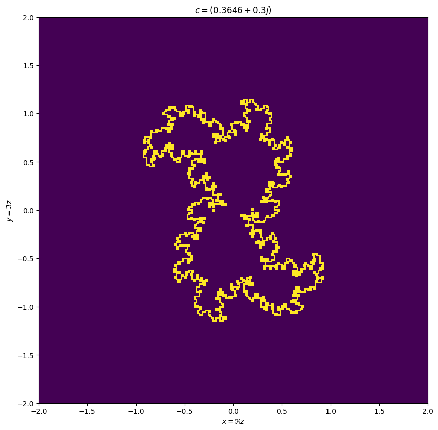
c = 0.3646 + 0.3j

# We will use a square box of length L = 2*Rx to make the counting easy.

Rx = 2
R = 4.0  # Bailout Radius

def compute(N, c=c, bailout=100, Rx=Rx):
    x = y = np.linspace(-Rx, Rx, N)
    X, Y = np.meshgrid(x, y)
    Z = X + 1j*Y
    outside = np.zeros(Z.shape, dtype=np.int64)
    
    for n in range(bailout):
        Z = np.where(np.logical_not(outside), Z**2 + c, Z)
        outside = np.where(np.logical_and(abs(Z) > R, np.logical_not(outside)), n, outside)
    inside = np.where(outside == 0, 1, 0)
    mean = (inside[1:,1:] + inside[1:,:-1] + inside[:-1,:-1] + inside[:-1,1:])
    J = np.where(np.logical_and(mean != 0, mean !=4), 1, 0)
    return result(x=x, y=y, J=J, inside=inside)
    
%time res = compute(256)
x, y, J = res.x, res.y, res.J
fig, ax = plt.subplots(1, 1, figsize=(10, 10))
#ax.pcolormesh(x, y, res.inside, shading="auto")#, cmap='Paired')
ax.pcolormesh(x, y, J)
ax.set(xlabel=r'$x=\Re z$', ylabel=r'$y=\Im z$', title=f"${c=}$");

CPU times: user 62.6 ms, sys: 28.7 ms, total: 91.3 ms
Wall time: 90.8 ms

../_images/244a141c12ab24bf4f178eb756600c48715997a8ea9a18cede9bf2932e14d4e2.png

BSM + Box Counting#

Using this approach, we can count the number of pixels that straddle the Julia set:

\[\begin{gather*} \DeclareMathOperator{\dim}{dim} d = \dim_{B} J = \lim_{\delta \rightarrow 0} \frac{\log N_{\delta}(J)}{-\log \delta}, \qquad \delta = \left(\frac{2R}{N}\right)^{2}, \qquad N_\delta \propto \frac{1}{\delta^{d}}. \end{gather*}\]

Ns = 2**np.arange(2, 11)
deltas = (2*R/Ns)**2
Ndeltas = [compute(N).J.sum() for N in Ns]
fig, ax = plt.subplots(1, 1)

# Asymptoic lower bound from Thm. 14.15 of Falconer:2014
dim = 2*np.log(2)/np.log(4*(abs(c) + np.sqrt(abs(2*c))))
ax.loglog(deltas, Ndeltas, '-x')
ax.plot(deltas, Ndeltas[-1]*(deltas[-1]/deltas)**dim, ':')
ax.set(xlabel=r"$\delta$", ylabel=r"$N_\delta$");

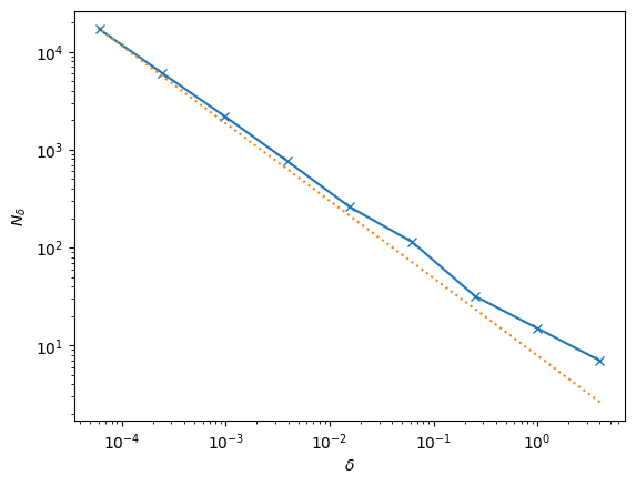
../_images/29f0de843b8977137a638c341e947982ff2c55038ba4f3fd367fcb3aa221352a.png

The lower bound given here (which appears to be a good approximation) is given in Theorem 14.15 of [Falconer, 2014].

Inverse Iteration Method#

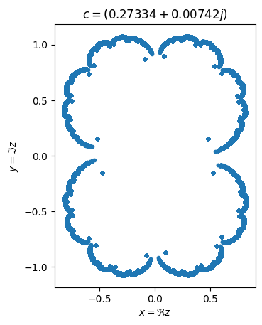
Another approach, the IIM - Inverse Iteration Method uses Theorem 14.10 of [Falconer, 2014], which notes that the inverse mapping \(f^{-1}(z)\) is attracted to \(J_c\). The algorithm is simply to randomly choose one of \(z\mapsto \pm \sqrt{z - c}\). We can start with either point \(z_0 = (1 \pm \sqrt{1-4c})/2 \in J_c\).

We start with the points produced by the BSM, then use a naïve IIM:

c = 0.27334 + 0.00742j

%time res = compute(256*4, c=c, bailout=2000)
x, y, J = res.x, res.y, res.J
fig, ax = plt.subplots(1, 1, figsize=(10, 10))
ax.pcolormesh(x, y, J)
ax.set(xlabel=r'$x=\Re z$', ylabel=r'$y=\Im z$', title=f"${c=}$");

def julia_IIM(c=c, N=12):
    zs = np.roots([1, -1, c])
    for n in range(N):
        d = np.sqrt(zs - c)
        zs = np.concatenate([zs, d, -d])
    return zs

%time zs = julia_IIM()

fig, ax = plt.subplots()
ax.plot(zs.real, zs.imag, '.')
ax.set(xlabel=r'$x=\Re z$', ylabel=r'$y=\Im z$', 
       title=f"${c=}$", aspect=1);

CPU times: user 27.8 s, sys: 37.2 ms, total: 27.8 s
Wall time: 27.8 s
CPU times: user 21.2 ms, sys: 4.03 ms, total: 25.2 ms
Wall time: 25.2 ms

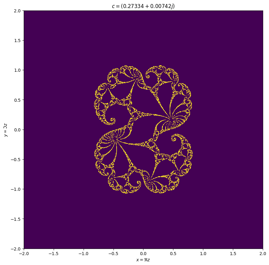
../_images/404dcc1be5bf113383fafe795dce9caa81db2e2d6849fb2636079868845a3b4a.png

../_images/13c9a30f0e68edd7f1635540e184606a75240517390c4556b47faa8668a4ebf0.png

Modified Inverse Iteration Method (Incomplete)#

As you can see, the points generated by the IIM do not uniformly sample the fractal. This is especially problematic for Julia sets near parabolic fixed points. The “deep” points are not visited nearly as frequently.

Newton Fractals#

Readings:

Newton’s Iteration and How to Abolish Two-Nation Boundaries in Chapter 1 of [Schroeder, 1991].
The Strange Sets of Julia and A Multifractal Julia Set in Chapter 11 of [Schroeder, 1991].
§4.17 of [Mattila, 1995].

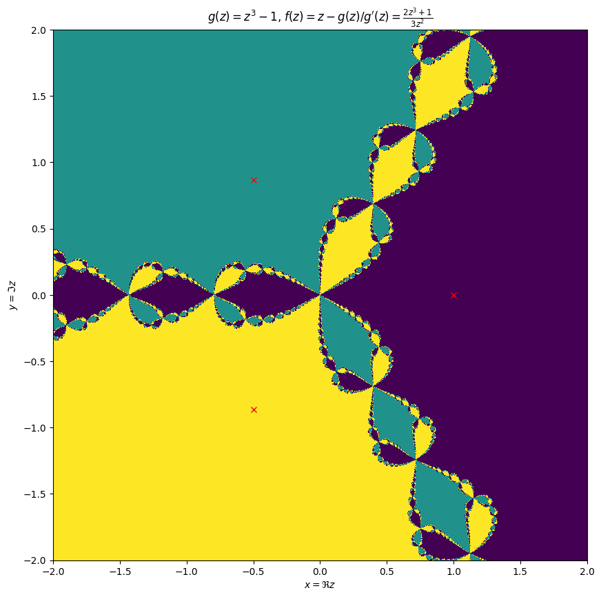
Consider Newton’s method for finding the complex roots of \(g(z) = z^{m} - 1 = 0\):

\[\begin{gather*} f_{m}(z) = z - \frac{g(z)}{g'(z)} = z - \frac{z^{m}-1}{mz^{m-1}} = z\left(1-\frac{1}{m}\right) + \frac{1}{mz^{m-1}}. \end{gather*}\]

Given an appropriate starting point, this should converge to one of the \(m\) roots \(p_{k} = e^{2\I \pi k /m}\), \(k \in \{0, 1, \dots, m-1\}\).

Do it! Find an \(\epsilon_{m}\) such that \(\abs{z_0-p_k}<\epsilon_{m}\implies z_n\rightarrow p_k.\)

Hint: Show that \(f_{m}(z)\) is a contraction mapping for \(z_0 = p_k + \epsilon\) with sufficiently small \(\epsilon\).

To produce a picture of the basins of attraction, one can simply iterate over the pixels in an image, computing the orbits, and bailing if the orbits contract appropriately. Try this now. Here is some code for \(m=3\).

import sympy

Nx, Ny = Nxy = (256*8,)*2
Rx, Ry = Rxy = (2, 2)
x, y = [np.linspace(-R, R, N) for R, N in zip(Rxy, Nxy)]
X, Y = np.meshgrid(x, y)
Z = X + 1j*Y

m = 3
k = np.arange(m)
p = np.exp(2j*np.pi * k/m)  # limit points
epsilon = 0.1

def g(z):
    return z**m - 1

# Here we use sympy to compute the Newton iteration.
z_ = sympy.var("z")
g_z_ = g(z_)
f_z_ = sympy.simplify(z_ - g_z_/g_z_.diff(z_))
f = sympy.lambdify(z_, f_z_, "numpy")
g_label = "g(z) = " + sympy.latex(g_z_)
f_label = "f(z) = z - g(z)/g'(z) = " + sympy.latex(f_z_)

assert(np.allclose(f(p), p))  # Check that limit points are invariant

fig, ax = plt.subplots(1, 1, figsize=(10, 10))
%time for n in range(55): Z = f(Z)

# Find the index of closest limit point (this will be the color).  This will
# be 0, 1, or 2 corresponding to the closest point p.
C = np.argmin(abs(Z[:, :, None] - p[None, None, :]), axis=-1)

ax.pcolormesh(x, y, C, shading="auto")
ax.plot(p.real, p.imag, 'rx')
ax.set(xlabel=r'$x=\Re z$', ylabel=r'$y=\Im z$', 
       title=f"${g_label}$, ${f_label}$");

CPU times: user 4.33 s, sys: 2.08 s, total: 6.41 s
Wall time: 6.41 s

../_images/89c909f69638b19040350a82f3c68e4bf43f8882dd87c59058e10ef61ac73638.png

Ideas for exploration:

We have hard-coded the limit points
Here we have manually chosen to iterate \(55\) times, and have used the analytic form for the limit points. Generalize your algorithm to work with any general function \(f(z)\) whose limit points are the fixed-points \(p = f(p)\) or applying Newton’s methjod to any function \(g(z)\) whose limit points are the roots \(g(p) = 0\).

Your algorithm will need to determine when your iteration has converged to a limit point, and will need to determine what the limit points are.

Applying the iteration to the entire array is not optimal from a computational perspective since some points converge quickly, while others (close to “the boundary”) converge more slowly.
Significant speed gains (at the expense of accuracy) can be achieved by employing methods to guess which regions should have the same color or by tracing the boundaries of these regions in pixel space (of course, the actual boundary is the Julia set, which is fractal, and thus has infinite length). Try playing with the XaoS application to get an idea of what is possible.

def color(Z, eps=0.1, nmax=1000):
    """Iterate until points stop moving and return the index of the nearest limit point."""
    for n in range(nmax):
        Z0, Z = Z, f(Z)
        if abs(Z - Z0).max() < eps:
            break
    C = np.argmin(abs(Z[:, :, None] - p[None, None, :]), axis=-1)
    return C, n
        
fig, axs = plt.subplots(5, 5)
for N, ax in enumerate(np.ravel(axs)):
    C = np.argmin(abs(Z[:, :, None] - p[None, None, :]), axis=-1)
    ax.imshow(C)
    ax.set(aspect=1)
    Z = f(Z)

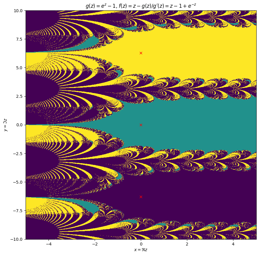
Figure 0.2: The Science of Fractal Images#

Here we apply the same techniques to get the background for Figure 0.2 in [Barnsley et al., 1988], which was used as the inside cover of Mandelbrot’s book.

\[\begin{gather*} g(z) = e^{z} - 1, \qquad z \mapsto f(z) = z - 1 + e^{-z}, \qquad p = \{2\pi n \I \mid n \in \mathbb{Z}\}. \end{gather*}\]

import sympy

Nx, Ny = Nxy = (256*4,256*8)
Rx, Ry = Rxy = (5, 10)
x, y = [np.linspace(-R, R, N) for R, N in zip(Rxy, Nxy)]
X, Y = np.meshgrid(x, y)
Z = X + 1j*Y

m = 1
k = np.arange(-m, m+1)
p = 2j*np.pi * k  # limit points
epsilon = 0.1

def g(z):
    return sympy.exp(z) - 1

# Here we use sympy to compute the Newton iteration.
z_ = sympy.var("z")
g_z_ = g(z_)
f_z_ = sympy.simplify(z_ - g_z_/g_z_.diff(z_))
f = sympy.lambdify(z_, f_z_, "numpy")
g_label = "g(z) = " + sympy.latex(g_z_)
f_label = "f(z) = z - g(z)/g'(z) = " + sympy.latex(f_z_)

assert(np.allclose(f(p), p))  # Check that limit points are invariant

%time for n in range(55): Z = f(Z)

# Find the index of closest limit point (this will be the color).  This will
# be 0, 1, or 2 corresponding to the closest point p.
C = np.argmin(abs(Z[:, :, None] - p[None, None, :]), axis=-1)

fig, ax = plt.subplots(1, 1, figsize=(10, 10))
ax.pcolormesh(x, y, C, shading="auto")

ax.plot(p.real, p.imag, 'rx')
ax.set(xlabel=r'$x=\Re z$', ylabel=r'$y=\Im z$', 
       title=f"${g_label}$, ${f_label}$");

<lambdifygenerated-2>:2: RuntimeWarning: overflow encountered in exp
  return z - 1 + exp(-z)
<lambdifygenerated-2>:2: RuntimeWarning: invalid value encountered in exp
  return z - 1 + exp(-z)
<lambdifygenerated-2>:2: RuntimeWarning: invalid value encountered in add
  return z - 1 + exp(-z)

CPU times: user 5.21 s, sys: 1.49 s, total: 6.7 s
Wall time: 6.7 s

../_images/4eea8ceb9aaa343eba1146ca2beb3fac2e7d1c5910a4c030899b752296337d6a.png