Show code cell content
import mmf_setup; mmf_setup.nbinit()
import os
from pathlib import Path
import logging; logging.getLogger("matplotlib").setLevel(logging.CRITICAL)
%matplotlib inline
import numpy as np, matplotlib.pyplot as plt
This cell adds /home/docs/checkouts/readthedocs.org/user_builds/iscimath-583-fractals/checkouts/latest/src to your path, and contains some definitions for equations and some CSS for styling the notebook. If things look a bit strange, please try the following:
- Choose "Trust Notebook" from the "File" menu.
- Re-execute this cell.
- Reload the notebook.
Assignment 2: Box Counting#
Determine a fractal dimension for some fractals by using the box-counting method.
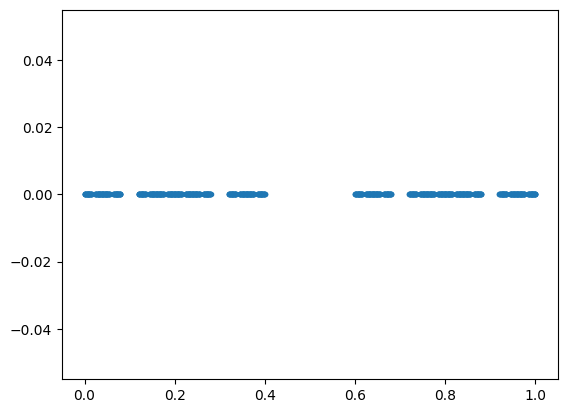
Here are some fractal for you to play with. (Please also make your own!) For now we restrict ourselves to 1D (i.e. the Cantor Set) or 2D in the complex plane.
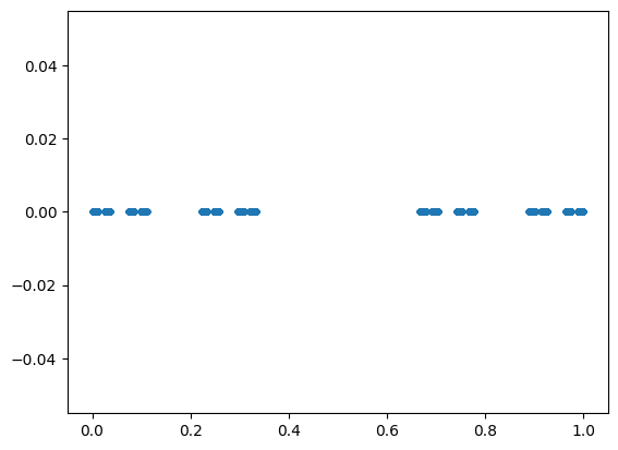
from math_583 import fractals

c = fractals.get_cantor(11)
plt.plot(c, 0*c, '.');
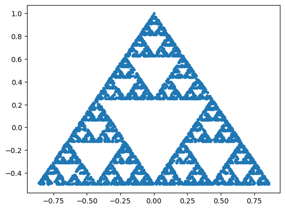
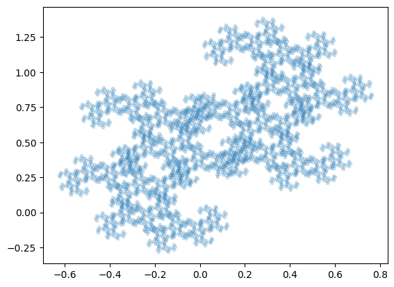
z = fractals.get_sierpinski(5000)
x, y = fractals.z2xy(z)
plt.plot(x, y, '.');
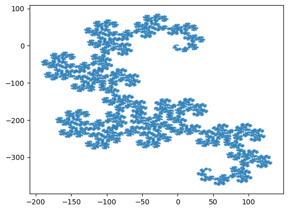
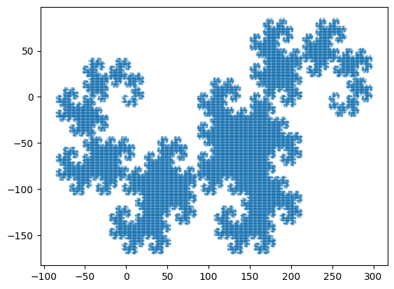
z = fractals.get_twindragon(100)
x, y = fractals.z2xy(z)
plt.plot(x, y, '.');
# Dragon curve
l = fractals.Lindenmayer(
    delta=90,
    axiom='F',
    F='F+G',
    G='F-G')
s = l.compute(16)

# We just draw the endpoints
z_dragon = np.concatenate(l.walk(s))
x, y = fractals.z2xy(z_dragon)
plt.plot(x, y, '.', ms=1, alpha=0.5);
Box Counting#
An easy way to perform the box counting is to use a histogram.
def count_box1(s, *v, **kw):
    """Return the number of boxes with points from `s`."""
    hist, x = np.histogram(s, *v, **kw)
    N = (hist > 0).sum()
    eps = np.mean(np.diff(x))
    return eps, N

def count_box2(z, *v, **kw):
    """Return the number of boxes with points from `x`."""
    z = np.asarray(z)
    hist, x, y = np.histogram2d(z.real, z.imag, *v, **kw)
    N = (hist > 0).sum()
    eps = np.mean(np.diff(x)) * np.mean(np.diff(y))
    return eps, N

print("Cantor Set: (box length, N)")
print(count_box1(c, bins=3))
print(count_box1(c, bins=3**2))
print(count_box1(c, bins=3**3))
print()
print("Dragon Curve: (box area, N)")
print(count_box2(z_dragon, bins=3))
print(count_box2(z_dragon, bins=3**2))
print(count_box2(z_dragon, bins=3**3))
Cantor Set: (box length, N)
(0.3333333333333333, 2)
(0.1111111111111111, 4)
(0.037037037037037035, 8)

Dragon Curve: (box area, N)
(10851.666666666668, 9)
(1205.7407407407409, 64)
(133.97119341563788, 440)
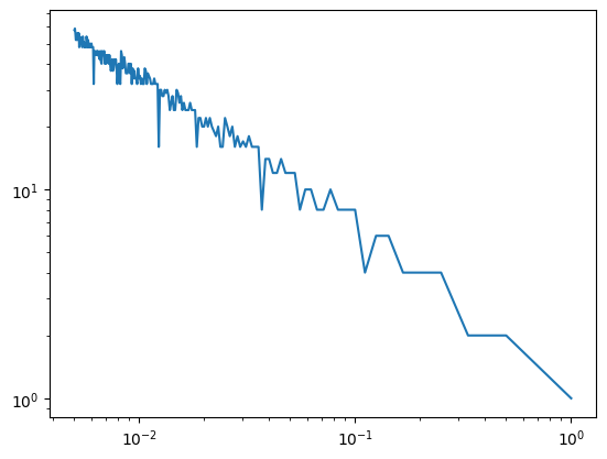
# The following might help:
epss = []
Ns = []
c = fractals.get_cantor(12)
Nbins = np.arange(1, 200)
for Nbin in Nbins:
    eps, N = count_box1(c, Nbin)
    epss.append(eps)
    Ns.append(N)

# Make these arrays in case you want to do arithmetic

epss, Ns = map(np.asarray, (epss, Ns))
plt.loglog(epss, Ns);
Visualization#
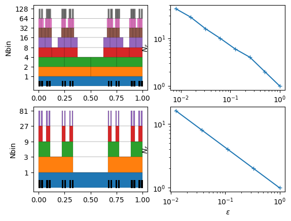
Here is some code to help visualize what is going on. The first plots the various filled boxes on top of each other in the 1D case.
from matplotlib.collections import LineCollection
def show_count1d(s, Nbins=(20,), ax=None, *v, **kw):
if ax is None:
ax = plt.gca()
epss = []
Ns = []
for n, Nbin in enumerate(Nbins):
hist, x = np.histogram(s, Nbin, *v, **kw)
epss.append(np.diff(x).mean())
Ns.append((hist > 0).sum())
dy = 1/len(Nbins)
y0 = n*dy
x, y = np.concatenate([[
(xl, 0), (xl, h*dy), (xh, h*dy), (xh, 0)]
for xl, xh, h in zip(x[:-1], x[1:], hist > 0)]).T
ax.fill_between(x, y0 + 0*y, y0 + y, ec='k', fc=f'C{n}', lw=0.1, alpha=1)
lines = np.array([[(x, 0), (x, dy/2)] for x in s])
ax.add_collection(LineCollection(lines, lw=0.5, alpha=0.5, color='k'))
ax.set(yticks=(1+np.arange(len(Nbins)))/len(Nbins),
yticklabels=Nbins,
ylabel="Nbin")
return epss, Ns
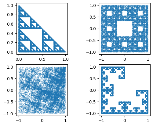
c = fractals.get_cantor(11)
fig, axs = plt.subplots(2, 2)
epss, Ns = show_count1d(c, 2**np.arange(8), ax=axs[0, 0]);
axs[0, 1].loglog(epss, Ns, '+-')
axs[0, 1].set(xlabel=r"$\epsilon$", ylabel=r"$N_{\epsilon}$")
epss, Ns = show_count1d(c, 3**np.arange(5), ax=axs[1, 0])
axs[1, 1].loglog(epss, Ns, '+-')
axs[1, 1].set(xlabel=r"$\epsilon$", ylabel=r"$N_{\epsilon}$");
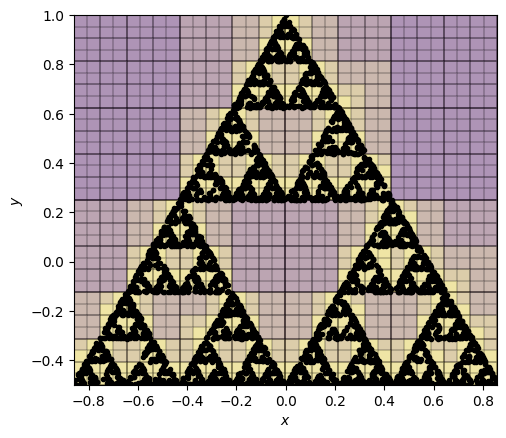
The second plots a image of the boxes.
from matplotlib.collections import LineCollection

def show_count2d(z, Nbins=(20,), ax=None, *v, **kw):
    z = np.asarray(z, dtype=complex)
    if ax is None:
        ax = plt.gca()
    epss = []
    Ns = []
    for n, Nbin in enumerate(Nbins):
        hist, x, y = np.histogram2d(z.real, z.imag, Nbin, *v, **kw)
        epss.append(np.diff(x).mean()*np.diff(y).mean())
        Ns.append((hist > 0).sum())
        ax.pcolormesh(x, y, (1+n)*(hist>0).T, edgecolors='k', linewidth=0.1, alpha=0.1)
    ax.plot(z.real, z.imag, 'k.')

    ax.set(xlabel="$x$", ylabel="$y$", aspect=1)
    return epss, Ns

z = fractals.get_sierpinski(5000)
epss, Ns = show_count2d(z, Nbins=2**(np.arange(1, 6)));
Fun Extensions#
For fun, we show some different fractals that you can generate with the code. How does the dimension change in these cases?
Cantor-like Sets#
The Cantor Set is generated as the proper fractions in a specified base
using only a specified set of allowed_digits. The standard set has base=3 and
allowed_digits=(0,2), but we can change this:
c = fractals.get_cantor(5, base=5, allowed_digits=(0,1,3,4))
plt.plot(c, 0*c, '.');
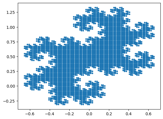
Twin Dragon#
The Twindragon is generated as the proper fractions in a specified complex
base=(1-1j), but you can change the base:
z = fractals.get_twindragon(100, base=(1.1-0.9j))
x, y = fractals.z2xy(z)
plt.plot(x, y, '.', alpha=0.2);
Other Gaskets (IFS)#
The Sir Pinski’s Game and Deterministic Chaos is generated as an iterated function system where we
randomly choose one of the three vertices attractors and move a specified fraction
weights towards each of these with specified probabilities. You can define your own
by changing these parameters. For example, here is “texture” defined by moving towards
each of the four vertices in a square, but with different probabilities. Note that this
does not change the dimension of the fractal.
The weights can be complex, allowing for rotations, or imperfect scaling to leave holes. This will affect the dimension.
args_sierpinski_gasket = dict(
    attractors=[0+0j, 0+1j, 1+0j],
    weights=1/2,
    probabilities=None)

args_sierpinski_carpet = dict(
    attractors=[(1+1j), (1+0j), (1-1j),
                (0+1j), #(0+0j),
                                 (0-1j),
                (-1+1j),(-1+0j), (-1-1j)],
    weights=2/3,
    probabilities=None)

args_square = dict(
    attractors=[(-1-1j), (1-1j), (-1+1j), (1+1j)],
    weights=1/2,
    rotations=[1, 1j, -1j, 1],
    probabilities=[1, 2, 1, 2])

# Variants of Fig. 5.21 in Peitgen's book. Not quite: we can't to flip (need conj()).
args_MRCM = dict(
    attractors=[-1-1j, 1-1j, -1+1j],
    weights=1/2,
    rotations=[1, 1j, -1j])

fig, axs = plt.subplots(2, 2)
for ax, args in zip(axs.ravel(), [args_sierpinski_gasket, args_sierpinski_carpet,
        args_square,  args_MRCM]):
    z = fractals.get_point_attractor(20000, **args)
    x, y = fractals.z2xy(z)
    ax.plot(x, y, '.', ms=1, alpha=0.5)
    ax.set(aspect=1);
L-systems#
The Lindenmayer systems L-Systems are very general. What happens if we don’t rotate by 90 degrees? Now we have something with lower dimension. How does the dimension depend on the angle?
# Dragon curve
l = fractals.Lindenmayer(
    delta=85,
    axiom='F',
    F='F+G',
    G='F-G')
s = l.compute(15)

# We just draw the endpoints
z_dragon = np.concatenate(l.walk(s))
x, y = fractals.z2xy(z_dragon)
plt.plot(x, y, '.', ms=1, alpha=0.5);