Show code cell content Hide code cell content

import mmf_setup; mmf_setup.nbinit()
import os
from pathlib import Path
import logging
logging.getLogger("matplotlib").setLevel(logging.CRITICAL)
logging.getLogger('numba').setLevel(logging.CRITICAL)
logging.getLogger('OMP').setLevel(logging.CRITICAL)
%matplotlib inline
import numpy as np, matplotlib.pyplot as plt

$\newcommand{\vect}[1]{\mathbf{#1}} \newcommand{\uvect}[1]{\hat{#1}} \newcommand{\abs}[1]{\lvert#1\rvert} \newcommand{\norm}[1]{\lVert#1\rVert} \newcommand{\I}{\mathrm{i}} \newcommand{\ket}[1]{\left|#1\right\rangle} \newcommand{\bra}[1]{\left\langle#1\right|} \newcommand{\braket}[1]{\langle#1\rangle} \newcommand{\Braket}[1]{\left\langle#1\right\rangle} \newcommand{\op}[1]{\mathbf{#1}} \newcommand{\mat}[1]{\mathbf{#1}} \newcommand{\d}{\mathrm{d}} \newcommand{\D}[1]{\mathcal{D}[#1]\;} \newcommand{\pdiff}[3][]{\frac{\partial^{#1} #2}{\partial {#3}^{#1}}} \newcommand{\diff}[3][]{\frac{\d^{#1} #2}{\d {#3}^{#1}}} \newcommand{\ddiff}[3][]{\frac{\delta^{#1} #2}{\delta {#3}^{#1}}} \newcommand{\floor}[1]{\left\lfloor#1\right\rfloor} \newcommand{\ceil}[1]{\left\lceil#1\right\rceil} % The following allows KaTeX to render these for significantly improved % performance on CoCalc. \newcommand{\DeclareMathOperator}[2]{\newcommand{#1}{#2}} \DeclareMathOperator{\Tr}{Tr} \DeclareMathOperator{\erf}{erf} \DeclareMathOperator{\erfi}{erfi} \DeclareMathOperator{\sech}{sech} \DeclareMathOperator{\sn}{sn} \DeclareMathOperator{\cn}{cn} \DeclareMathOperator{\dn}{dn} \DeclareMathOperator{\sgn}{sgn} \DeclareMathOperator{\order}{O} \DeclareMathOperator{\diag}{diag} % \newcommand{\mylabel}[1]{\label{#1}\tag{#1}} \newcommand{\degree}{\circ}$

This cell adds /home/docs/checkouts/readthedocs.org/user_builds/iscimath-583-fractals/checkouts/latest/src to your path, and contains some definitions for equations and some CSS for styling the notebook. If things look a bit strange, please try the following:

• Choose "Trust Notebook" from the "File" menu.
• Re-execute this cell.
• Reload the notebook.

Assignment 9: Newton’s Method

Suppose you need to find the roots of a function \(g(z) = 0\) numerically. One common solution to problems of this type is to use Newton’s method. Newton’s method is an iterative algorithm

\[\begin{gather*} z_{n+1} = f(z_{n}), \qquad f(z) = z - \frac{g(z)}{g'(z)}. \end{gather*}\]

Recall that a fixed-point is superstable if the derivative vanishes \(f'(z) = 0\) at the fixed-point. Newton’s iteration is superstable at the roots of \(g(z) = 0\), so if \(z_{n}\) is sufficiently close to the root, the iteration will rapidly converge, roughly doubling the number of correct digits with each iteration.

Do it! Show that the roots are superstable fixed-points of \(z=f(z)\).

Differentiating, we have:

\[\begin{gather*} f'(z) = 1 - \frac{g'(z)}{g'(z)} + \frac{g(z)g''(z)}{\bigl(g'(z)\bigr)^2} = \frac{g(z)g''(z)}{\bigl(g'(z)\bigr)^2}. \end{gather*}\]

Thus, \(f'(z) = 0\) if \(g(z) = 0\), i.e., if \(z\) is a root of \(g(z)\), unless \(g'(z) = 0\), in which case, we might have a problem.

One challenge lies in choosing a suitable initial guess \(z_{0}\) to ensure rapid convergence. Often one can find an algorithm for choosing a good initial guess to ensure that one has a globally convergent Newton’s method that works for all input parameters.

from math_583.newton import NewtonWeb

def g(z, d=0):
    """Return the dth derivative of the function."""
    if d == 0:
        return z**3 - 1
    else:
        return 3*z**2
        
fig, ax = plt.subplots()
NewtonWeb(g, x0=-2.0).draw(ax=ax);

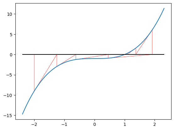
To get an idea of which initial guesses \(z_{0}\) will converge rapidly to a root, we might try counting how many iterations \(n\) it takes until \(\abs{g(z_n)} < \epsilon\) is less than some specified tolerance.

Polynomials

This assignment assumes you have watched the two videos about this topic by 3Blue1Brown:

As discussed in the videos by 3Blue1Brown, one application of Newton’s method is to find the roots of polynomials. By the fundamental theorem of algebra, we can express any polynomial \(g(z)\) up to an overall constant as a product of its roots \(\vect{r} = \{r_i\}\):

\[\begin{gather*} g(z) = \prod_{i} (z-r_i). \end{gather*}\]

The corresponding Newton iteration can thus be expressed as

\[\begin{gather*} f(z) = z - \frac{g(z)}{g'(z)} = z - \frac{1}{\sum_{i} \frac{1}{z-r_i}},\\ f'(z) = \frac{g(z)g''(z)}{\bigl(g'(z)\bigr)^2} \end{gather*}\]

Do it! Show that this form of \(f(z)\) is correct.

This follows from applying the product rule:

\[\begin{gather*} g'(z) = \sum_{i}\prod_{j\neq i}(z-r_i) = \sum_{i} \frac{g(z)}{z-r_i},\\ g''(z) = \sum_{i} \frac{g'(z)}{z-r_i} - \sum_{i} \frac{g(z)}{(z-r_i)^2} = \sum_{i} \frac{g'(z)(z-r_i) - g(z)}{(z-r_i)^2} = g(z)\sum_{i} \frac{\sum_{j}\frac{(z-r_i)}{z-r_j} - 1}{(z-r_i)^2}\\ = g(z)\sum_{ij} \frac{r_j - r_i}{(z-r_j)(z-r_i)^2}\\ \end{gather*}\]

Here we implement Newton’s method using a slight modification of our escape-time algorithm, converging instead when \(\abs{g(z_{n})} \leq \epsilon\) is less than some small number.

Show code cell source Hide code cell source

%matplotlib inline
import numpy as np, matplotlib.pyplot as plt
import numba

# Since we want to pass in the roots as an array, we must generalize and use
# guvectorize, which means we must write our own loop.  Note also that even scalar
# arguments must be arrays
@numba.guvectorize(
    ["(complex128[:,:], complex128[:], float64[:], int_[:], int32[:,:])"],
    "(m,n),(i),(),()->(m,n)",
    cache=True,
    target="parallel",
)
def _convergence_time(z0, roots, eps, maxiter, n):
    for x in range(z0.shape[0]):
        for y in range(z0.shape[1]):
            z = z0[x, y]
            for n[x, y] in range(maxiter[0] + 1):
                g = 1 + 0j
                tmp = 0j
                for r_i in roots:
                    g *= (z-r_i)
                    tmp += 1/(z-r_i)
                z -= 1/tmp
                if g.real**2 + g.imag**2 <= eps[0]:
                    break

def convergence_time(z0, roots, eps=1e-8, maxiter=100):
    """Return the "convergence time" of initial point `z0` under Newton's method.

    Arguments
    ---------
    z0 : complex
        Location in the Julia set.
    roots : complex array
        Roots of the polynomial.
    eps : float
        Bailout radius.
    maxiter : int
        Maximum number of iteration.  If the iteration does not terminate before this,
        then this value is returned.  It can be used as an approximation of the interior
        of the sets.
    """
    return _convergence_time(z0, roots, eps, maxiter)


# Try changing the ranges here
x = np.linspace(-2, 2, 1024)
y = np.linspace(-2, 2, 1024)
z = x[:, None] + 1j*y[None, :]

roots = np.exp(2j*np.pi * (np.arange(3)/3.0))

# Try changing maxiter - especially if you get deep.
%time n = convergence_time(z, roots, maxiter=1000)

fig, ax = plt.subplots()
mesh = ax.pcolormesh(x, y, n.T, shading='auto')
fig.colorbar(mesh, label=r"Convergence time $n$")
ax.set(xlabel=r"$x = \Re z$", ylabel=r"$y = \Im z$", 
       title=f"Newton convergence time for $g(z)=z^3-1$.",  aspect=1);

CPU times: user 334 ms, sys: 0 ns, total: 334 ms
Wall time: 320 ms

This is in fact not an analogy with Julia sets, but is an example of a Julia set as originally studied by Julia and Fatou. Their work concerned rational functions \(z\mapsto Q(z)\) and thus includes Newton’s iteration for polynomials. For example, in the case shown

\[\begin{gather*} f(z) = Q(z) = \frac{2z^3+1}{3z^2}. \end{gather*}\]

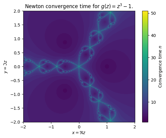
Notice that, in analogy with the filled Julia sets \(K_c\), there is a set of measure zero that does not converge, forming a fractal boundary between the basins of attraction. In this example, for \(g(z) = z^3 - 1\), the filled Julia set coincides with the Julia set \(J_{\vect{r}} = \partial K_{\vect{r}} = K_{\vect{r}}\) – i.e. there are no interior points. But as discussed in the second video, if you choose the roots \(\vect{r}\) carefully then interior points can open up.

Main Tasks

Find a polynomial \(g(z)\) where \(K_{\vect{r}}\) has interior points and then modify the code to draw the corresponding Mandelbrot set.

Formally, you are looking for polynomials where the Newton iteration has a attractive cycle (of period > 1). The mathematically inclined might like to prove that if there is such a cycle, then it will contain the geometric mean of the roots:

\[\begin{gather*} \bar{r} = \frac{1}{N_i}\sum_{i=1}^{N} r_i \end{gather*}\]

Lambert \(W\) Function

For example, the Lambert \(W\) function arises in the exact solution of the double delta-function potential problem in 1D quantum mechanics.

Suppose you need to solve the following equation for \(w\):

\[\begin{gather*} z = w e^w, \qquad w = W(z). \end{gather*}\]

This is called the Lambert \(W\) function.

w = np.linspace(-4, 2, 500)
z = w*np.exp(w)
fig, ax = plt.subplots()
ax.plot(z, w)
w = np.linspace(-1, 2, 500)
z = w*np.exp(w)
ax.plot(z, w, lw=4)
ax.grid()
ax.set(ylim=(-4, 2), xlim=(-1, 6),
       xlabel="$z$", ylabel="$w=W(z)$", title="Lambert $W$ function");

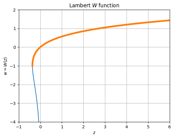
For the purposes of this assignment, your challenge is to compute this accurately for the upper branch (thick orange curve) where \(w\geq -1\) and \(z\geq -1/e\), sometimes labeled \(w = W_{0}(z)\) (with \(w = W_{-1}(z)\) being the lower blue branch).

One common solution to problems of this type (inverse problems) is to use Newton’s method, which can be expressed in terms of finding the root(s) of a function \(g(z) = 0\). Newton’s method is an iterative algorithm

\[\begin{gather*} z_{n+1} = f(z_{n}), \qquad f(z) = z - \frac{g(z)}{g'(z)}. \end{gather*}\]

Recall that a fixed-point is superstable if the derivative vanishes \(f'(z) = 0\) at the fixed-point. Newton’s iteration is superstable at the roots of \(g(z) = 0\), so if \(z_{n}\) is sufficiently close to the root, the iteration will rapidly converge, roughly doubling the number of correct digits with each iteration.

Do it! Show that the roots are superstable fixed-points of \(z=f(z)\).

Differentiating, we have:

\[\begin{gather*} f'(z) = 1 - \frac{g'(z)}{g'(z)} + \frac{g(z)g''(z)}{\bigl(g'(z)\bigr)^2} = \frac{g(z)g''(z)}{\bigl(g'(z)\bigr)^2}. \end{gather*}\]

Thus, \(f'(z) = 0\) if \(g(z) = 0\), i.e., if \(z\) is a root of \(g(z)\), unless \(g'(z) = 0\), in which case, we might have a problem.

One challenge lies in choosing a suitable initial guess \(z_{0}\) to ensure rapid convergence. Often one can find an algorithm for choosing a good initial guess to ensure that one has a globally convergent Newton’s method that works for all input parameters (\(w \in [-1, \infty]\) in our case).

Do it! Find a globally convergent Newton’s method for \(W(z)\).

Some hints:

• Typically one has problems in the asymptotic regions. In this case, you will probably have difficulty converging for either large \(w\) or for \(w\approx -1\). Can you use asymptotic expansions (I.e. Taylor series) to help you get a good guess in either region?

• You do not need to apply Newton’s method to the original \(g(z)=0\). Sometimes rearranging the equation can help. For example, suppose you are trying to find the roots of the polynomial \(z^6 + z = 1\). You might rewrite this as \(g(z) = z - (1 - z)^(1/6) = 0\) and apply Newton’s method.

• It can be helpful to make a plot as a function of the input parameters, the number of iterations \(N\) your algorithm requires to reach a fixed desired tolerance \(\abs{g(z)} \leq \epsilon\). This can help you choose an algorithm depending on the value of the inputs. (Note: “your algorithm” here include both the heuristic for estimating \(z_0\) and the Newton’s iteration. You may need to adjust both in some regions of parameter space.)

Solution

Not yet.

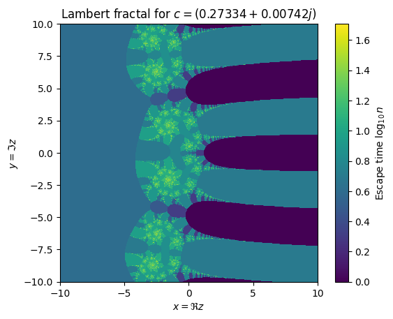
Lambert Fractal

One can define several fractals based on the Lambert function. Here is a start, using the escape-time algorithm with “escape” defined as \(\Re z_{n} > 4\) for the iteration \(z\mapsto ze^z + c\). This does not consider the possibility of fixed points or cycles. Can you generalize? If you get something worthwhile, please [contribute to Wikipedia][Lambert W function], where there is an outstanding request for such a picture.

Ideas to explore include:

• Is there a corresponding “Mandelbrot” set?

• What does the Newton fractal look like?

%matplotlib inline
import numpy as np, matplotlib.pyplot as plt

@numba.vectorize(
    ["int32(complex128, complex128, float64, int_)"],
    cache=True,
    target="parallel",
)
def _escape_time_Lambert(c, z0=0j, R=4.0, maxiter=100):
    z = z0
    for n in range(maxiter + 1):
        z = z * np.exp(z) + c
        if z.real > R:
            break
    return n


def escape_time_Lambert(c, z0=0j, R=4.0, maxiter=100):
    """Return the "escape time" of initial point `z0` under `z->z*exp(z)+c`.

    Arguments
    ---------
    c : complex
        Parameter defining the Julia set or location in the Mandelbrot set.
    z0 : complex
        Location in the Julia set or parameter defining the Mandelbrot set.  (For values
        of `z0 != 0`, one gets a different Mandelbrot-like set.)
    R : float
        Bailout "radius".
    maxiter : int
        Maximum number of iteration.  If the iteration does not terminate before this,
        then this value is returned.  It can be used as an approximation of the interior
        of the sets.
    """
    return _escape_time_Lambert(c, z0, R, maxiter)


# Try changing the ranges here
x = np.linspace(-10, 10, 1024)
y = np.linspace(-10, 10, 1024)
z = x[:, None] + 1j*y[None, :]

# Try playing with different values of c
c = 0.27334+0.00742j

# Try changing maxiter - especially if you get deep.
%time n = escape_time_Lambert(c, z, maxiter=1000)

fig, ax = plt.subplots()
mesh = ax.pcolormesh(x, y, np.log10(1+n).T, shading='auto')
fig.colorbar(mesh, label=r"Escape time $\log_{10} n$")
ax.set(xlabel=r"$x = \Re z$", ylabel=r"$y = \Im z$", 
       title=f"Lambert fractal for $c={c}$",
       aspect=1);

CPU times: user 330 ms, sys: 0 ns, total: 330 ms
Wall time: 175 ms

References