HPC Assignment 1: Percolation#

Review Chapter 15 in [Schroeder, 1991]: Percolation: From Forest Fires to Epidemics. Reproduce the figures in the textbook, and [Albinet et al., 1986] for a square lattice with nearest-neighbor interactions (Sq in Fig. 2 of [Albinet et al., 1986]). Specifically, calculate the percolation threshold \(P_c \approx 0.593\) numerically in this case.

First write a short algorithm that gets you in the ballpark with [CoCalc][] or your laptop. [Albinet et al., 1986] considers grids of size up to 300×300, so you should be able to use the methods there to calculate three digits.

I think that the statistical errors should be easy to understand, but the systematic errors might be more challenging.
Numerical convergence on a value for \(P_c\) will have both statistical errors that can be reduced by performing more trials, and systematic errors from the finite size of your lattice. Determine how your accuracy depends on both of these factors by performing some experiments varying both the lattice size and number of samples. Do you understand theoretically where the scaling you observe comes from?
Ensure that you method can be scaled up to use larger computer (Kamiak in our case). Don’t try scaling yet, but think about your approach and make sure it is feasible.
Estimate how accurately you can determine \(P_c\) using a supercomputer. What will be the limiting factors (memory? wall-time? communication?).
Estimate by how much you can improve your estimate of \(P_c\) by optimizing your code. How much do you think you can improve your code by using a faster language? Tools like Numba (if using Python) etc.?
Now estimate your time: what can you do in a couple of hours? A couple of days? A couple of months? Do this both for your current state of knowledge, and your idea of what you could accomplish once you have some experience optimizing code, writing and running code on a cluster, etc. Where is it most worth you investing effort to improve your ability to solve such problems?
If it makes sense, then try to improve your estimate of \(P_c\) using Kamiak. (Even if it does not make sense, you might want to use this problem to just get some experience running code on Kamiak, but it would be better to do it for a problem that will actually benefit.) Note: if you really need accuracy, it is usually better to think carefully about your algorithm – you will not get exponential gains by moving to an HPC platform, but sometimes can with a better algorithm. However, this might take a lot more of your time, so turning to HPC resources might still make sense if you have access.

Followup questions:

Apparently at threshold, the burn front has a fractal dimension. What is this dimension?
What happens if the burn starts at a single site rather than along one edge? Does the front have the same fractal dimension?

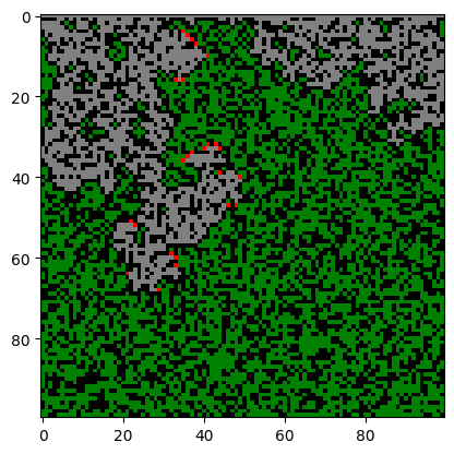
A Rough Start#

Here is a simple code. It is very slow…

from itertools import product
from matplotlib.colors import ListedColormap

Nx, Ny = Nxy = (100, 100)
rng = np.random.default_rng(seed=2024)
pc = 0.5927460507921

# 0: No tree
# 1: Living tree
# 2: Burning tree
# 3: Burnt tree

X = rng.choice(2, size=Nxy, p=[1-pc, pc])

# Make slightly large array to add ghost-points to simplify testing
X0_ = np.zeros((Nx+2, Ny+2))
X0_[1:-1, 1:-1] = X
X0_[1, 1:-1] = 2   # Burning top row

# Some plotting routines
cm = ListedColormap(["black", "green", "red", "grey"])
def draw(X_, ax=None):
    if ax is None:
        ax = plt.gca()
    ax.imshow(X_[1:-1, 1:-1], cmap=cm, vmin=0, vmax=3)

def update(X_):
    Nx, Ny = X_[1:-1, 1:-1].shape
    Xnew_ = X_.copy()
    for nx, ny in product(range(1, Nx+1), range(1, Ny+1)):
        # If tree is alive and any neighbours on fire...
        if (X_[nx, ny] == 1 and any(np.array(
                [X_[nx-1, ny], X_[nx+1, ny], X_[nx, ny-1], X_[nx, ny+1]]) == 2)):
            Xnew_[nx, ny] = 2  # New tree is on fire.
        elif X_[nx, ny] == 2:  # If tree is on fire
            Xnew_[nx, ny] = 3  # New tree is burnt.
    return Xnew_

X_ = X0_
%time for n in range(100): X_ = update(X_)
draw(X_)

CPU times: user 2.51 s, sys: 1.53 ms, total: 2.51 s
Wall time: 2.51 s

../_images/47b23a8447bf1eebcde70540ddaec5a2016f3293540fe0a1a4974bb7039b8784.png

How can we make this faster? Some ideas:

Try to vectorize the calculation. (Can we do a convolution with rounding?)
Only trace burning trees?
Use Numba.
Hashlife?

Let’s try a combination of vectorization and iterating over burning sites only:

def update1(X_):
    Nx, Ny = X_[1:-1, 1:-1].shape
    Xnew_ = X_.copy()
    burning = np.where(X_ ==  2)
    Xnew_[burning] = 3
    for ix, iy in zip(*burning):
        for d in (-1, +1):
            if X_[ix+d, iy] == 1:
                Xnew_[ix+d, iy] = 2
            if X_[ix, iy+d] == 1:
                Xnew_[ix, iy+d] = 2
    return Xnew_

X_ = X0_
%time for n in range(100): X_ = update1(X_)
draw(X_)

CPU times: user 9.85 ms, sys: 137 µs, total: 9.99 ms
Wall time: 9.43 ms

How about Numba?

from numba import njit, prange

@njit(parallel=True)
def update3(X_):
    Nx, Ny = X_[1:-1, 1:-1].shape
    X1_ = X_.copy()
    for nx in prange(1, Nx+1):
        for ny in range(1, Ny+1):
            if X_[nx, ny] == 2:  # If tree is on fire
                 X1_[nx, ny] = 3  # New tree is burnt.
            elif (X_[nx, ny] == 1 
                and (X_[nx-1, ny] == 2 
                     or X_[nx+1, ny] == 2 
                     or X_[nx, ny-1] == 2 
                     or X_[nx, ny+1] == 2)):
                 X1_[nx, ny] = 2
    return X1_

X_ = X0_.copy()
update3(X_);  # Compile once
%time for n in range(100): X_ = update3(X_)
draw(X_)

CPU times: user 1.38 ms, sys: 113 µs, total: 1.49 ms
Wall time: 1.49 ms

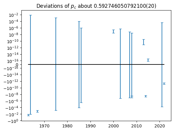
Statistical Analysis#

To test your code, it is good to have an idea of what the correct answer might be. The Wikipedia entry on percolation thresholds lists the following values with errors. Are these statistically consistent?

from uncertainties import ufloat, ufloat_fromstr, unumpy as unp

data = [
    (1963, '0.569(13)'),
    (1964, '0.590(10)'), 
    (1967, '0.591(1)'),
    (1975, '0.593(1)'),
    (1985, '0.59274(10)'), 
    (1986, '0.592745(2)'),
    (2000, '0.59274621(13)'), 
    (2003, '0.59274621(33)'), 
    (2007, '0.59274603(9)'), 
    (2008, '0.59274598(4)'), 
    (2008, '0.59274605(3)'), # Wiki [30] 10.1103/PhysRevE.76.027702, 
                             #      [31] 10.1103/PhysRevE.78.031131
    (2013, '0.59274605095(15)'), 
    (2014, '0.59274601(2)'),   # Wiki 10.1088/1751-8113/47/13/135001
    (2015, '0.59274605079210(2)'), 
    (2021, '0.59274(5)'), # Wiki [35]: 10.1103/PhysRevE.103.012115
    (2022, '0.592746050786(3)'),
]

yrs = np.array([date for date, num in data])
ps = np.array([ufloat_fromstr(num) for date, num in data])

n_, s_ = unp.nominal_values, unp.std_devs 
p, dp = n_(ps), s_(ps)

# Compute the weighted mean
w = 1/dp**2
p_mean = sum(ps*w)/sum(w)

fig, ax = plt.subplots()
ax.errorbar(yrs, n_(ps-p_mean), s_(ps-p_mean), capsize=3, ls='none')
ax.set_yscale('symlog', linthresh=1e-16)
ax.plot(yrs, 0*yrs, 'k')
ax.set(title=f"Deviations of $p_c$ about {p_mean:S}");

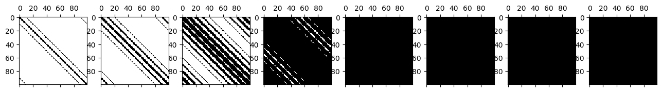
../_images/ff557ab3016fd916a8628a6f2ed4d0c0b699c38f70f445ab0e78342e9d723bb0.png

Adjacency Matrix#

Another approach is to use the adjacency matrix \(\mat{A}\). The idea here is that \(A_{ij}\) represents the number of edges connecting vertex \(i\) to vertex \(j\). Note that these are directed, if the edge also allows one to move from \(j\) to \(i\), then this needs to go in \(A_{ji}\). Thus, if the edges are not directed, the adjacency matrix should be symmetric \(\mat{A} = \mat{A}^T\). One may also include loops by specifying diagonal elements.

The nice property of the adjacency matrix is that \(\mat{A}^n\) describes the connectivity after taking \(n\) steps. Since there are generally multiple ways to move around, the entries in \(\mat{A}^n\) will get large, so we can consider connectivity by simply setting all positive values to 1 after. We can also speed the process of creating the connections by repeatedly squaring the matrix, which needs to be done at most \(\log_2 N\) times where there are \(N\) vertices.

The only remaining challenge is to construct the appropriate adjacency matrix \(\mat{A}\) for our desired grid. Consider an \(M\times N\) grid. We can label the cells “lexicographically” as \(i = n + mN\), m = i//N, n=i%N:

M, N = 2, 3
m, n = np.arange(M)[:, None], np.arange(N)[None, :]
v = n + m*N
display(v.ravel())
display(v)
display(v % N)
display(v // N)

array([0, 1, 2, 3, 4, 5])

array([[0, 1, 2],
       [3, 4, 5]])

array([[0, 1, 2],
       [0, 1, 2]])

array([[0, 0, 0],
       [1, 1, 1]])

Here we use a function get_neighbours(m, n, M, N) to fill in the adjacency matrix.

def get_neighbours(i, M, N, periodic=True):
    """Return a list of the neighbours to point `i`."""
    neighbours = []
    m, n = i // N, i % N
    if m == 0:
        if periodic:
            neighbours.append((M-1, n))
    else:
        neighbours.append((m-1, n))
        
    if n == 0:
        if periodic:
            neighbours.append((m, N-1))
    else:
        neighbours.append((m, n-1))
    
    if m == M-1:
        if periodic:
            neighbours.append((0, n))
    else:
        neighbours.append((m+1, n))

    if n == N-1:
        if periodic:
            neighbours.append((m, 0))
    else:
        neighbours.append((m, n+1))
    
    neighbours = [n + m*N for (m, n) in neighbours]
    return neighbours

get_neighbours(1, 2, 3)

def plot(A, M, N, ax=None):
    if ax is None:
        fig, ax = plt.subplots()
    else:
        fig = ax.figure
        
    for i, j in zip(*np.where(A)):
        mi, ni = i // N, i % N
        mj, nj = j // N, j % N
        ax.plot([mi, mj], [ni, nj], '-k')
    ax.set(aspect=1)

Now we can form the adjacency matrix:

M, N = 10, 10
A = np.zeros((M*N, M*N), dtype=bool)
for i in range(N*M):
    n = get_neighbours(i, M=M, N=N)
    A[i, i] = A[i, n] = A[n, i] = True
assert np.allclose(A, A.T)
As = [A]
for n in range(int(np.ceil(np.log2(N*M)))):
    As.append(As[-1] @ As[-1])

fig, axs = plt.subplots(1, len(As), figsize=(len(As)*2, 2))
for _A, ax in zip(As, axs):
    ax.spy(_A);

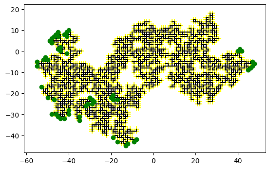
../_images/c35f0a5a120f304a5e6414824b60eb124d524c87ca65693249023438a81e6ff2.png

Another Approach#

In the previous approaches, we pick an initial grid, then look at percolation from the top to the bottom. This might introduce finite-size effects.

Here we try another approach. We start at a cell and then randomly build out the network, choosing links or cells randomly from the burn front. This way, we only need to keep track of the cells which are alive or have been burned. This should be significantly more efficient if we are well below the percolation threshold, and allows us to extend to arbitrary sizes.

For variation, we consider here the bond-percolation threshold, which will be proven in class to be \(p_c=1/2\).

from matplotlib.colors import ListedColormap
from matplotlib.collections import LineCollection


class Percolation:
    cm = ListedColormap(["yellow", "black"])
    seed = 2
    initial_cells = ((0, 0), )
    p = 0.4

    def __init__(self, **kw):
        for key in kw:
            if not hasattr(self, key):
                raise ValueError(f"Unknown {key=}")
            setattr(self, key, kw[key])
        self.init()

    def init(self):
        self.rng = np.random.default_rng(seed=self.seed)
        self.links = {}
        self.cells = set(self.initial_cells)
        self.front = list(self.cells)

        # stages is a list of (new_links, front)
        self.stages = [(dict(self.links), list(self.front))]

    def get_neighbours(self, cell):
        """Return the neighbours of cell that have not been visited."""
        x, y = cell
        neighbours = [
            n for n in [(x + 1, y), (x - 1, y), (x, y + 1), (x, y - 1)]
            if n not in self.cells
        ]
        return neighbours

    def bounds(self):
        """Return the bounds.  (Suitable for plt.axis().)"""
        A = np.array(list(self.cells))
        x0, y0 = A.min(axis=0)
        x1, y1 = A.max(axis=0)
        return (x0, x1, y0, y1)

    def step(self):
        """Evolve the simulation one step forward."""
        new_front = []
        new_links = {}
        if not self.front:
            return

        for cell in self.front:
            for new_cell in self.get_neighbours(cell):
                link = tuple(sorted([cell, new_cell]))
                if link not in self.links:
                    connected = self.rng.random() < self.p
                    new_links[link] = connected
                    if connected:
                        new_front.append(new_cell)
        self.front = set(new_front)
        self.cells.update(self.front)
        self.links.update(new_links)
        self.stages.append((new_links, list(self.front)))

    def plot_network(self, stage=None, lines=None, ax=None):
        if ax is None:
            fig, ax = plt.subplots()
        else:
            fig = ax.figure

        connected_lines = []
        broken_lines = []

        if stage is None:
            stage = -1
        links, front = self.stages[stage]

        for link in links:
            line = [link[0], link[1]]
            if links[link]:
                connected_lines.append(line)
            else:
                broken_lines.append(line)
        if lines is None:
            lc0 = LineCollection(broken_lines,
                                 ls='-',
                                 color=self.cm(0),
                                 zorder=0)
            lc1 = LineCollection(connected_lines,
                                 ls='-',
                                 color=self.cm(1),
                                 zorder=1)
            l3, = ax.plot(*np.transpose(front), 'o', c='green')
            ax.add_collection(lc0)
            ax.add_collection(lc1)
            ax.set(aspect=1)
            ax.axis(self.bounds())
            lines = (lc0, lc1, l3)
        else:
            lc0, lc1, l3 = lines
            broken_lines.extend(lc0.get_segments())
            connected_lines.extend(lc1.get_segments())
            lc0.set_segments(broken_lines)
            lc1.set_segments(connected_lines)
            l3.set_data(np.transpose(front))

        ax.axis(self.bounds())

        return lines, ax

Ns = 100
steps = 1000
ps = np.linspace(0.4, 0.49, 10)
results = []
for _p in ps:
    res = np.zeros(2)
    for sample in range(Ns):
        p = Percolation(p=_p, seed=2+sample)
        for step in range(steps):
            if not p.front:
                break
            p.step()
        # msg = f"{step=}, {len(p.front)=}, {len(p.cells)=}"
        # clear_output(wait=True)
        # display(msg)
        res += [len(p.cells), len(p.stages)]
    res /= Ns
    results.append(res)

results = np.asarray(results)

fig, ax = plt.subplots()
ax.plot(np.log10(abs(ps-0.5)), np.log10(results))
ax.legend(labels=["cluster size", "time"])

<matplotlib.legend.Legend at 0x7ff028606510>

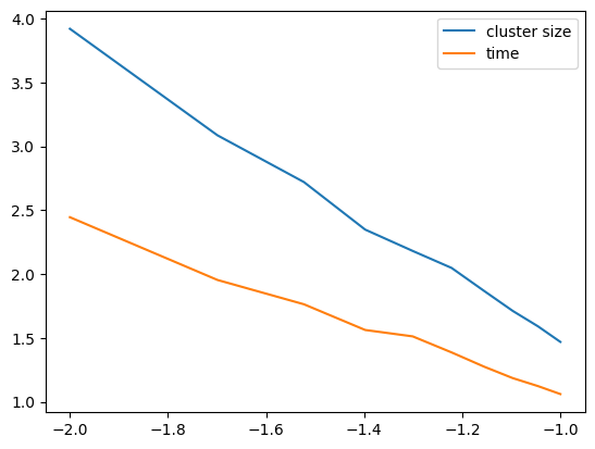
../_images/bf8bbcb55ee0a591bc0f645787efff5b6299979ff78ce63718ac0c7f884b9b47.png

from scipy.optimize import curve_fit

def f(p, a, pc, gamma):
    return a + gamma*np.log10(abs(p-pc))

display(curve_fit(f, ps, np.log10(results[:, 0]), p0=(0, 1, -2.0))))
display(curve_fit(f, ps, np.log10(results[:, 1]), p0=(0, 1, -2.0))))

  Cell In[11], line 6
    display(curve_fit(f, ps, np.log10(results[:, 0]), p0=(0, 1, -2.0))))
                                                                       ^
SyntaxError: unmatched ')'

cm = ListedColormap(["yellow", "black"])

rng = np.random.default_rng(seed=2)


def get_neighbours(cell):
    global cells, links
    x, y = cell
    neighbours = [n for n in [(x+1, y), (x-1, y), (x, y+1), (x, y-1)] 
                  if n not in cells]
    return neighbours


def plot_network(links, front, ax=None):
    if ax is None:
        fig, ax = plt.subplots()
    fig = ax.figure
    for link in links:
        connected = links[link]
        ax.plot(*list(zip(link[0], link[1])), '-', c=cm(connected), zorder=connected)
    for cell in front:
        ax.plot([cell[0]], [cell[1]], 'o', c="green")
    ax.set(aspect=1)
    return fig


p = 0.49
max_steps = 100

links = {}
cells = {(0,0)}
front = [(0,0)]
stages = [(dict(links), list(front))]

for n in range(max_steps):
    new_front = []
    for cell in front:
        for new_cell in get_neighbours(cell):
            link = tuple(sorted([cell, new_cell]))
            if link not in links:
                connected = links[link] = rng.random() < p
                if connected:
                    new_front.append(new_cell)
    front = new_front
    stages.append((dict(links), list(front)))

fig, ax = plt.subplots()
plot_network(links=links, front=front, ax=ax);
axis = ax.axis()

../_images/b2e2e4967315c53be6d33ee2d8bd6a338a21ff6bdc0cf73f41eccdd1b40efe92.png

One can animate this process, but re-drawing the network each time gets slow as the number of links becomes large. To speed this up, we use a matplotlib.collections.LineCollection

from matplotlib.animation import FuncAnimation
from IPython.display import HTML, display

fig, ax = plt.subplots()

def draw(ax=ax):
    for links, front in stages:
        ax.cla()
        plot_network(links=links, front=front, ax=ax)
        ax.set(axis=axis)
        yield ax

animation = FuncAnimation(
    fig,
    draw,
    frames=stages,
    interval=80,
    init_func=draw,
    blit=False,
)

display(HTML(animation.to_jshtml()))
plt.close("all")

References:#

[Schroeder, 1991]: Chapter 15 – Percolation: From Forest Fires to Epidemics
[Albinet et al., 1986]: Ref. [ASS 86] in [Schroeder, 1991].
[Stauffer and Aharony, 1994]: Revised 2nd Edition of Ref. [Sta 85] in [Schroeder, 1991].

HPC Assignment 1: Percolation

Contents