Show code cell content
import mmf_setup; mmf_setup.nbinit()
import os
from pathlib import Path
FIG_DIR = Path(mmf_setup.ROOT) / '../Docs/_build/figures/'
os.makedirs(FIG_DIR, exist_ok=True)
import logging; logging.getLogger("matplotlib").setLevel(logging.CRITICAL)
%matplotlib inline
import numpy as np, matplotlib.pyplot as plt
try: from myst_nb import glue
except: glue = None
This cell adds /home/docs/checkouts/readthedocs.org/user_builds/iscimath-583-fractals/checkouts/latest/src to your path, and contains some definitions for equations and some CSS for styling the notebook. If things look a bit strange, please try the following:
- Choose "Trust Notebook" from the "File" menu.
- Re-execute this cell.
- Reload the notebook.
Mandelbrot Set#
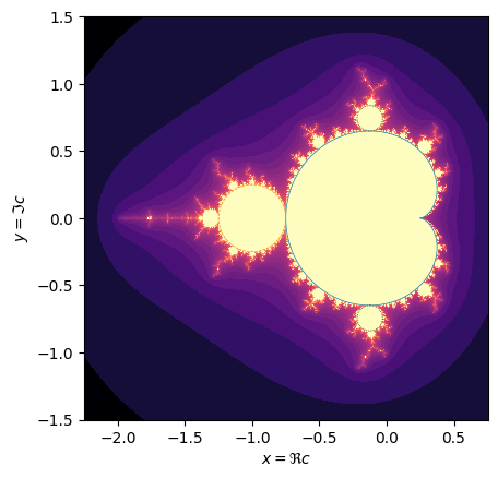
The Mandelbrot set \(M\) is the set of all points \(c\) such that the iteration \(f: z \mapsto z^2+c\) remains bounded starting from \(z_0 = 0\). It turns out that corresponding Julia sets \(J_c\) are connected and have finite measure.
We can approximate the Mandelbrot set with the same escape-time algorithm as for the Julia sets, but instead of fixing \(c\), we now let \(c \in \mathbb{C}\) vary over the plane, and fix the initial point \(z_0 = 0+0\I\). In this sense, \(M\) describes what happens to the origin of \(K_c\), the filled-in Julia set: if \(c\in M\), then \(0 \in K_c\) and vice versa. It turns out that if \(c \in M\), then \(J_c\) and \(K_c\) are connected.
from math_583.mandelbrot import escape_time

def get_mandelbrot(c=-0.75, r=1.5, Nx=256*4, Ny=None, maxiter=100, z0=0, ax=None):
    """Draw M centered on `c` with radius `c+-r`."""
    x = np.linspace(c.real-r, c.real+r, Nx)
    if Ny is None:
        Ny = Nx
    ry = Ny*r/Nx
    y = np.linspace(c.imag-ry, c.imag+ry, Ny)
    z = x[:, None] + 1j*y[None, :]
    res = escape_time(c=z, z0=z0)
    return x, y, res

x, y, M = get_mandelbrot()
fig, ax = plt.subplots()
ax.pcolormesh(x, y, np.log(1+M).T, cmap='magma')
ax.set(aspect=1, xlabel=r"$x=\Re c$", ylabel="$y=\Im c$");

phi = np.linspace(0, 2*np.pi, 1000)
q = np.exp(1j*phi)
c1 = q*(2-q)/4
c2 = q/4 - 1

# From {cite}`Giarrusso:1995`
w = np.arcsinh((88-27*q)/80/np.sqrt(5))/3
c3s = [-7/4 - 20/9*(np.sinh(w + 2j*k*np.pi/3) - 1/4/np.sqrt(5))**2
       for k in [0, 1, 2]]
ax.plot(c1.real, c1.imag, '-', lw=0.5)
ax.plot(c2.real, c2.imag, '--', lw=0.5)
for c3 in c3s:
    ax.plot(c3.real, c3.imag, ':k', lw=0.5)
A Surprise#
In 1991, while exploring the point \(c=-3/4\) at the neck between the main cardioid and the largest bulb, David Boll stumbled on the following surprise. He was trying to see if this neck was infinitely thin, and so exploring the escape-times for points \(c = -3/4 + \I \epsilon\) along the imaginary axis when he found this series:
eps = 1/10**np.arange(8)

[escape_time(c=-3/4+eps*1j, R=4.0, maxiter=1000000000) for eps in eps]
[3, 33, 315, 3143, 31417, 314160, 3141593, 31415927]
He also approached the butt of the main cardioid \(c=1/4 + \epsilon\) where he found this:
eps = 1/10**np.arange(13)

[escape_time(c=1/4+eps, R=4.0, maxiter=1000000000) for eps in eps]
[2, 8, 30, 97, 312, 991, 3140, 9933, 31414, 99344, 314157, 993457, 3141625]
This second example is simpler since the iteration is purely real (and was know significantly earlier as a property of tangent bifurcations. See [Peitgen et al., 2004] and references therein.
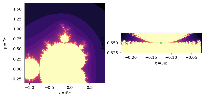
Question: Does a similar phenomenon happen at \(c=(-1 + 3\sqrt{3}\I)/8\)?
(Incomplete)
This point is on the not so trivial: if one simply parameterizes
then the escape time fluctuates rapidly \(c\) passes in and out of \(M\). Instead, we must move along a path midway between the main cardioid \(c_1\) and tertiary bulb \(c_3\). The main cardioid \(c_1\) and secondary bulb \(c_2\) have simple forms (see Julia Sets), but the tertiary bud requires solving a cubic [Giarrusso and Fisher, 1995].
Suggestion: use the results of [Giarrusso and Fisher, 1995] (or derive your own) to find a
second-order approximation to both the main cardioid c_1 and the tertiary bulb c_3
at \(c\), and then approach long the midpoint between these.
To find \(c_3\) one can look for the solutions to the following two equations, additionally factoring out the period 1 solutions:
s = 2*np.pi/3
q = np.exp(1j*s)
c = q*(2-q)/4
fig, axs = plt.subplots(1, 2, figsize=(8, 4))

ax = axs[0]
x, y, M = get_mandelbrot(c, r=1)
ax.pcolormesh(x, y, np.log(1+M).T, cmap='magma')
ax.plot([c.real], [c.imag], 'xg')
ax.set(aspect=1, xlabel=r"$x=\Re c$", ylabel="$y=\Im c$");

ax = axs[1]
x, y, M = get_mandelbrot(c, r=0.1, maxiter=2000, Nx=1024, Ny=256)
ax.pcolormesh(x, y, np.log(1+M).T, cmap='magma')
ax.plot([c.real], [c.imag], 'xg')
ax.axhline([c.imag], ls=':', c='g')
ax.set(aspect=1, xlabel=r"$x=\Re c$", ylabel="$y=\Im c$");