Show code cell content
import mmf_setup; mmf_setup.nbinit()
import os
from pathlib import Path
import logging
logging.getLogger("matplotlib").setLevel(logging.CRITICAL)
logging.getLogger('numba').setLevel(logging.CRITICAL)
logging.getLogger('OMP').setLevel(logging.CRITICAL)
%matplotlib inline
import numpy as np, matplotlib.pyplot as plt
This cell adds /home/docs/checkouts/readthedocs.org/user_builds/iscimath-583-fractals/checkouts/latest/src to your path, and contains some definitions for equations and some CSS for styling the notebook. If things look a bit strange, please try the following:
- Choose "Trust Notebook" from the "File" menu.
- Re-execute this cell.
- Reload the notebook.
Assignment 3: Julia Set#
The goal of this assignment is to sample points in a Julia set \(J_c\) for \(z^2+c\) for various values of the parameter \(c\). From these samples, you should use your program to compute a fractal dimension.
Concrete Problem Statement#
For those of you who like a concrete problem statement, implement the following function:
def julia_sample(c, N):
    """Return a list of `N` points from the Julia set `J_c`."""
This can then be used to estimate the fractal dimension of \(J_c\) using box counting for example, as demonstrated in Boundary Scanning Method (BSM).
Exploration#
To get a feel for the structure of Julia sets, you can play with the following code. This uses a compiled version of the escape-time algorithm which you should implement below. For now, you can play a bit:
%matplotlib inline
import numpy as np, matplotlib.pyplot as plt
from math_583.mandelbrot import escape_time
# Try changing the ranges here
x = np.linspace(-2, 2, 1024)
y = np.linspace(-2, 2, 1024)
z = x[:, None] + 1j*y[None, :]
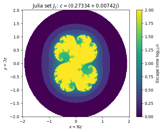
# Try playing with different values of c
c = 0.27334+0.00742j
# Try changing maxiter - especially if you get deep.
%time n = escape_time(c, z, maxiter=100)
fig, ax = plt.subplots()
mesh = ax.pcolormesh(x, y, np.log10(n).T, shading='auto')
fig.colorbar(mesh, label=r"Escape time $\log_{10} n$")
ax.set(xlabel=r"$x = \Re z$", ylabel=r"$y = \Im z$",
title=f"Julia set $J_c$: $c={c}$",
aspect=1);
CPU times: user 127 ms, sys: 0 ns, total: 127 ms
Wall time: 64.3 ms
/tmp/ipykernel_3646/2452525088.py:19: RuntimeWarning: divide by zero encountered in log10
  mesh = ax.pcolormesh(x, y, np.log10(n).T, shading='auto')

The code here works, but the UX is a bit cludgy. You might want to instead download
XaoS and play with it. Note: the default there is to explore the [Mandelbrot set][]
\(M\), which we will do next assignment. The set \(M\) provides a classification for the
different Julia sets. To see the corresponding Julia set \(J_c\), use the m
(Mandelbrot/Julia switching) or j (Fast Julia preview mode) keyboard shortcuts .
Coding Suggestions#
Escape-Time Algorithm#
Here is a simple python version of the previous algorithm. It is very slow, but you can have complete control over it. Can you think how to make the algorithm faster (not simply by compiling)? If you have any substantial improvements, we can work with you to implement those in a compiled version.
def julia_escape_time(c,
                      R=4.0, maxiter=100,
                      x_range=(-2, 2), y_range=(-2, 2), Nx=200, Ny=200):
    """Return `(x, y, res)` where `res` is the number iterations to "escape".

    Arguments
    ---------
    R : float
        Bailout radius.  We say that a point has "escaped" once `abs(z) > R`.
    maxiter : int
        Maximum number of iterations.  We say that a point has not escaped if `abs(z) < R`
        for `maxiter` iterations.  Such points provide an approximation of the filled-in
        Julia set `K_c` and will have `n == maxiter`.

    c : complex
        Parameter defining the Julia set for $z^2+c$.
    x_range, y_range : (float, float)
        Range to plot: `x_range = (x[0], x[-1])` etc.
    Nx, Ny : int
        Number of pixels in each direction.  `res.shape == (Nx, Ny)`.

    Results
    -------
    x, y : float arrays
        1D arrays of the cell boundaries.  Note that these should have `Nx` and `Ny`
        elements because they are cell boundaries.  See the code below for how to do this.
    res : 2D int array
        This is an array of integers expressing how many iterations it takes the initial
        point `z=x+j*y` to escape `abs(z) > R`.  Note that `res.shape = (Nx, Ny)`.
    """

    # Some code to get you started... but feel free to explore other techniques.
    x = np.linspace(*x_range, Nx)  # These are the pixel centers, not the boundaries.
    y = np.linspace(*y_range, Ny)
    res = np.zeros((Nx, Ny), dtype=int)

    # Your code here.  Possibly something based on the following loop, but this will be
    # slow.  I recommend starting with a loop, but then trying to vectorize or optimize
    # your code later.
    for nx in range(Nx):
        for ny in range(Ny):
            #######################
            # Calculate res[nx, ny]
            #
            # Your code here, but this works.
            z = x[nx] + 1j*y[ny]
            for n in range(maxiter + 1):
                z = z**2 + c
                if abs(z) > R:
                    break
            res[nx, ny] = n
    return x, y, res
Here is how this function could be used to generate the plot above:
c = 0.27334+0.00742j
args = dict(c=c, maxiter=100,
            x_range=(-2, 2), y_range=(-2, 2),
            Nx=256, Ny=256)
%time x, y, res = julia_escape_time(**args)

fig, ax = plt.subplots()
# Shading needed when x, y give cell centers instead of boundaries
# The transpose is because we are not using meshgrid (image/MATLAB compatibility).
mesh = ax.pcolormesh(x, y, np.log10(res).T, shading='auto')
fig.colorbar(mesh, label=r"Escape time $\log_{10} n$")
ax.set(xlabel=r"$x = \Re z$", ylabel=r"$y = \Im z$",
       title=f"Julia set $J_c$: $c={c}$",
       aspect=1);
CPU times: user 400 ms, sys: 29 µs, total: 400 ms
Wall time: 400 ms
/tmp/ipykernel_3646/1988924678.py:10: RuntimeWarning: divide by zero encountered in log10
  mesh = ax.pcolormesh(x, y, np.log10(res).T, shading='auto')
BSM - Boundary Scanning Method#
The previous escape-time algorithm is useful for determining the filled-in Julia sets \(K_c\), but for computing the fractal dimension, we are really interested in the Julia set itself \(J_c = \partial K_c\), which is the boundary. (In most cases, \(\mathrm{dim} K_c = 2\) which is uninteresting.)
The goal here is to determine whether or not a cell \((x, y) \in [x_0, x_1] \times [y_0, y_1]\) contains an element \(z \in J_c\) of the Julia set.
def get_julia(c, x_range=(-2, 2), y_range=(-2, 2), Nx=200, Ny=200):
    """Return `(x, y, res)` where `res` is 1 if the corresponding cell contains points in $J_c$.

    Arguments
    ---------
    c : complex
        Parameter defining the Julia set for $z^2+c$.
    x_range, y_range : (float, float)
        Range to plot: `x_range = (x[0], x[-1])` etc.
    Nx, Ny : int
        Number of pixels in each direction.  `res.shape == (Nx, Ny)`.

    Results
    -------
    x, y : float arrays
        1D arrays of the cell boundaries.  Note that these should have `Nx+1` and `Ny+1`
        elements because they are cell boundaries.  See the code below for how to do this.
    res : 2D bool array
        This is 1 where the corresponding cell contains points of the Julia set and 0
        elsewhere.  Note that `res.shape = (Nx, Ny)`.
    """

    # Some code to get you started... but feel free to explore other techniques.
    x = np.linspace(*x_range, Nx+1)  # Add one extra point for boundaries
    y = np.linspace(*y_range, Ny+1)
    res = np.zeros((Nx, Ny), dtype=bool)  # Bool arrays save a little space.

    # Your code here.  Possibly something based on the following loop, but this will be
    # slow.  I recommend starting with a loop, but then trying to vectorize or optimize
    # your code later.
    for nx in range(Nx):
        for ny in range(Ny):
            x0, x1 = x[nx:nx+2]   # Boundary of cell.
            y0, y1 = y[ny:ny+2]

            #####################
            # Calculate f[nx, ny]
            #
            # Your code here.
            res[nx, ny] = True

    return x, y, res
Once you have this working, you should be able to apply the BSM Box counting technique.