Show code cell content
import mmf_setup; mmf_setup.nbinit()
import os
from pathlib import Path
import logging
logging.getLogger("matplotlib").setLevel(logging.CRITICAL)
logging.getLogger('numba').setLevel(logging.CRITICAL)
logging.getLogger('OMP').setLevel(logging.CRITICAL)
%matplotlib inline
import numpy as np, matplotlib.pyplot as plt
This cell adds /home/docs/checkouts/readthedocs.org/user_builds/iscimath-583-fractals/checkouts/latest/src to your path, and contains some definitions for equations and some CSS for styling the notebook. If things look a bit strange, please try the following:
- Choose "Trust Notebook" from the "File" menu.
- Re-execute this cell.
- Reload the notebook.
Assignment 8: Feigenbaum Constant Revisited#
Let us revisit the computation of the Feigenbaum constant. From Assignment 6: Feigenbaum Constant and the Logistic Map you should have been able to at least estimate this from the location of the bifurcation points \(r_{n}\) where the period doubles to \(2^n\), but computing these is a little tricky. [Schroeder, 1991] suggests a better approach in Chapter 12 section Self Similarity in the Logistic Parabola using the values of \(r=R_{2^n}\) that give superstable orbits of period \(2^n\).
Stability#
Consider a fixed-point \(x\) such that \(f(x) = x\). Perturbing this we have
Thus, the fixed-point is attractive if \(\abs{f'(x)} < 1\), repulsive if \(\abs{f'(x)} > 1\), and indeterminant if \(\abs{f'(x)} = 1\). A stable fixed point will attract nearby points. A fixed-point is superstable if \(f'(x) = 0\). This notion can be applied to orbits of period \(n\), i.e. fixed points of \(x = f^{(n)}(x)\).
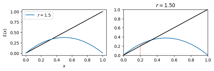
Question 1: Find \(R_1\)#
Find parameter values \(R_{1}\) that give rise to a superstable fixed-point of period \(1\). Demonstrate numerically that this point is indeed exhibits very fast convergence.
R1 = 1.5 # WRONG! Put in the correct value
%matplotlib inline
import numpy as np, matplotlib.pyplot as plt

from math_583.plotting import CobWeb

plt.rcParams['figure.figsize'] = (5, 3)

def f(x, r, d=0):
    """Logistic growth function (or derivative)"""
    if d == 0:
        return r*x*(1-x)
    elif d == 1:
        return r*(1-2*x)
    elif d == 2:
        return -2*r
    else:
        return 0


x = np.linspace(0, 1)
fig, axs = plt.subplots(1, 2, figsize=(8, 2))
ax = axs[0]

ax.plot(x, x, '-k')
ax.plot(x, f(x, r=R1), label=f"$r={R1}$")
ax.legend()
ax.set(xlabel="$x$", ylabel="$f_r(x)$");

CobWeb(f).cobweb(r=R1, ax=axs[1]);
# Maybe this will help.  It should converge in about 7 steps, with extremely
# rapid convergence once it gets close if you have the correct value for R1

r = R1
xs = [0, 0.2]
while abs(np.diff(xs[-2:])) > 1e-12 and len(xs) < 100:
    x = xs[-1]
    xs.append(r*x*(1-x))
    print(x)
0.2
0.24000000000000005
0.27360000000000007
0.29811456000000003
0.3138634036740096
0.323029751262263
0.3280222965925552
0.33063550429605143
0.3319735013924208
0.3326506436485158
0.33299128939311595
0.3331621358721391
0.3332476906398802
0.3332905009846003
0.3333119144070516
0.3333226231820369
0.3333279780856241
0.3333306556664607
0.3333319944891422
0.333332663908549
0.33333299862026894
0.33333316597663315
0.3333332496549412
0.3333332914941267
0.3333333124137274
0.3333333228735297
0.33333332810343136
0.3333333307183823
0.33333333202585774
0.3333333326795955
0.33333333300646434
0.3333333331698989
0.3333333332516161
0.33333333329247467
0.33333333331290405
0.3333333333231187
0.33333333332822596
0.3333333333307796
0.3333333333320565
Solution
We look for solutions to the equations
Solving for \(R_n\)#
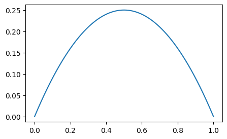
You should have found that the superstability condition \(f'(x) = 0\) gives \(x_0 = 1/2\). Argue that \(x_0 = 1/2\) must be in the superstable orbits of higher period.
I.e., let
Argue that, if you find a period \(n\) fixed point such that \(x_n = x_0\), then the condition that the orbit is superstable
implies that the point \(1/2\) is on the orbit. We will start here \(x_0 = 1/2\).
# Play with this, or make your own plot, and convince yourself that
# the derivative of f^(n)(1/2) is always zero.
try:
    from ipywidgets import interact
except ImportError:
    # On ReadTheDocs, we disable interact
    def interact(**kw):
        def wrapper(f):
            f()
        return wrapper

@interact(r=(1.0, 4.0), n=(1, 20))
def draw(r=1.0, n=1):
    x = x0 = np.linspace(0, 1, 1000)
    for _n in range(n):
        x = f(x, r)
    plt.plot(x0, x)
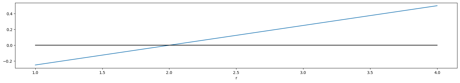
This gives us a strategy. We simply look for roots of the objective function as a function of \(r\).
def objective(r, n):
    """Return f^n(1/2) - 1/2."""
    x = 0.5
    for _n in range(n):
        x = r*x*(1-x)
    return x - 1/2


@interact(n=(1, 20), a=(1.0, 4.0, 0.001), b=(1.0, 4.0, 0.001))
def draw(n=1, a=1.0, b=4.0):
    fig, ax = plt.subplots(figsize=(20,3))
    r = np.linspace(a, b, 1000)
    ax.plot(r, objective(r, n))
    ax.plot(r, 0*r, 'k')
    ax.set(xlabel="r")
A Systematic Approach#
Consider the equation \(f^{(2)}{}'(x) = 0\) first to find a point on the orbit, then compute \(r\).
Solution
We are now looking for solutions to the equations
The second equation still has the solution \(x=1/2\) as before, so this point must be on the orbit. This point iterates to:
This same reasoning holds for any value of \(n\). We then have
You saw from the previous assignment that the logistic map appeared to be chaotic for \(r=4\):
Staisław Ulam and John von Neumann suggested using this as a way of generating pseudo-random numbers. Your task is to explore how well this works and try to improve the naïve implementation.
References#
Section A Case of Complete Chaos in Chapter 12 of [Schroeder, 1991].
Section 5.1: The Multiple Reduction Copy Machine Metaphor of Peitgen et al. “Chaos and Fractals: New Frontiers of Science” (Online acces through WSU Library.)
Section 6.4: Random Number Generator Pitfall of Peitgen et al. Chaos and Fractals: New Frontiers of Science (Online acces through WSU Library.)
Wikipedia: Logistic Map: Solutions when \(r=4\).