Show code cell content
import mmf_setup; mmf_setup.nbinit()
import os
from pathlib import Path
import logging
logging.getLogger("matplotlib").setLevel(logging.CRITICAL)
logging.getLogger('numba').setLevel(logging.CRITICAL)
logging.getLogger('OMP').setLevel(logging.CRITICAL)
%matplotlib inline
import numpy as np, matplotlib.pyplot as plt
This cell adds /home/docs/checkouts/readthedocs.org/user_builds/iscimath-583-fractals/checkouts/latest/src to your path, and contains some definitions for equations and some CSS for styling the notebook. If things look a bit strange, please try the following:
- Choose "Trust Notebook" from the "File" menu.
- Re-execute this cell.
- Reload the notebook.
Assignment 7: Pseudo-Random Numbers#
You saw from the previous assignment that the logistic map appeared to be chaotic for \(r=4\):
Staisław Ulam and John von Neumann suggested using this as a way of generating pseudo-random numbers. Your task is to explore how well this works and try to improve the naïve implementation.
References#
Section A Case of Complete Chaos in Chapter 12 of [Schroeder, 1991].
Section 5.1: The Multiple Reduction Copy Machine Metaphor of Peitgen et al. “Chaos and Fractals: New Frontiers of Science” (Online acces through WSU Library.)
Section 6.4: Random Number Generator Pitfall of Peitgen et al. Chaos and Fractals: New Frontiers of Science (Online acces through WSU Library.)
Wikipedia: Logistic Map: Solutions when \(r=4\).
Motivation: MRCM and the Sierpiński Gasket#
Many fractals can be sampled by the method of inverse iteration whereby we sample points in the fractal by randomly iterating from a series of contractive maps. This is called the Multiple Reduction Copy Machine (MRCM) in [Peitgen et al., 2004] which is an alternative way of specifying iterated function systems (MRCM = IFS). As we discussed before, the Sierpinski gasket can be generated by picking three points \(\{p_0, p_1, p_2\}\) in a triangle, and collecting samples by randomly moving half-way towards any of these points.
To do this requires a way of randomly choosing the index \(n \in \{0, 1, 2\}\) with equal probability, for which we turn to a pseudo-random number generator. NumPy has a pretty good one (based on PCG64.)
%matplotlib inline
import numpy as np, matplotlib.pyplot as plt
import scipy.stats, scipy as sp

plt.rcParams['figure.figsize'] = (5, 3)

def get_sierpinski(y):
    """Return samples in he Sierpinski gasket using the random numbers y."""

    # Fixed points in an equilateral triangle
    thetas = 2*np.pi * (np.arange(3)/3 + 1/4)
    ps = np.exp(1j*thetas)

    p = ps[0]   # Start with one point.
    ns = np.floor(3*y).astype(int)
    res = [p]
    for n in ns:
        p1 = ps[n]  # Choose one of the three points randomly
        p = (p + p1)/2  # Move half-way to p1.
        res.append(p)
    return np.array(res)

rng = np.random.default_rng(seed=2)

Ns = 10000
y = rng.random(Ns)
p = get_sierpinski(y)
fig, ax = plt.subplots()
ax.plot(p.real, p.imag, '.', ms=0.5)
ax.set(aspect=1, xlabel="x", ylabel="y");

Roll-your-own Random Number Generator#
Let’s see if we can use the chaotic orbits from the \(r=4\) logistic map \(x\mapsto
4x(1-x)\) to generate pseudo random numbers? We start with get_random_x() which
simply returns \(N\) samples \(x_n\) from the orbit. As we shall see, these are not
uniform, but being clever, we can then transforming them to a new variable \(y_n\) such
that the distribution is uniform on [0, 1]. Your task is to try to understand why this
transformation works, then test the quality of the map as a way to generate random
numbers. As you might guess from the title of some of the references, these
pseudo-random numbers are poor in some cases.
def get_random_x(N, x0=np.sqrt(2)):
    """Return N pseudo-random numbers between 0 and 1.

    Arguments
    ---------
    N : int
        Number of pseudo-random numbers to generate.
    x0 : float
        Seed to start the generator.  Must be chosen carefully.
    """
    x = x0 % 1  # The mod operator % makes sure initial point is 0 <= x0 < 1.
    xs = [x]
    while len(xs) < N:
        x = 4*x*(1-x)
        xs.append(x)
    return np.array(xs)

def get_uniform(N, x0=np.sqrt(2)):
    """Return N uniformly distributed numbers between 0 and 1."""
    x = get_random_x(N=N, x0=x0)
    y = 0.5 - np.arcsin(1-2*x)/np.pi
    return y
Examples#
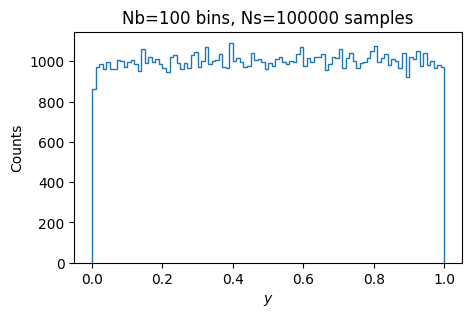
Here we generate some histograms and related plots that you might use to test the quality of the random numbers. Your task is to come up with some ways to quantify how uniform the generator is. Can you choose a “bad” seed?
Nb = 100     # Number of bins equally spaced between 0 and 1
Ns = 100000  # Number of samples.
y = get_uniform(N=Ns)
h, bins = np.histogram(y, bins=Nb, range=(0, 1))  # Histogram
fig, ax = plt.subplots()
ax.stairs(h, bins)
ax.set(xlabel="$y$", ylabel="Counts", title=f"{Nb=} bins, {Ns=} samples");
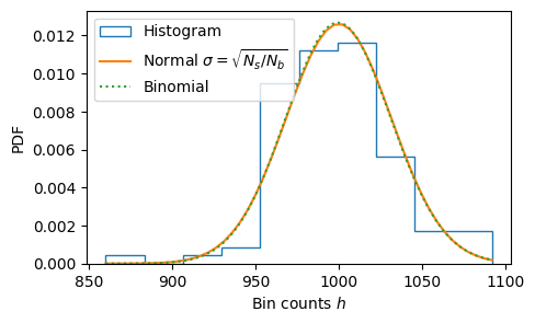
You might like to look at the distribution of the fluctuations. Are these consistent with what you would expect for a uniform distribution?
fig, ax = plt.subplots()
ax.hist(h, bins=len(h)//10, density=True, histtype='step', label="Histogram")
ax.set(xlabel="Bin counts $h$", ylabel="PDF");

# Is this a gaussian?  (No, but it is a good approximation for large N)
# Why is this variance correct?
h_ = np.linspace(h.min(), h.max())
rv = sp.stats.norm(loc=Ns/Nb, scale=np.sqrt(Ns/Nb))
ax.plot(h_, rv.pdf(h_), label=r"Normal $\sigma=\sqrt{N_s/N_b}$")

# Is this a binomial distribution?  (Yes... why?)
rv = sp.stats.binom(Ns, p=1/Nb)
h_ = np.arange(h.min(), h.max())
ax.plot(h_, rv.pmf(h_), ':', label="Binomial")

ax.legend();
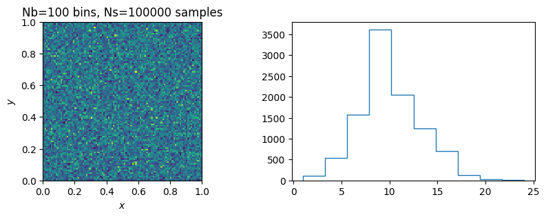
You might also look in 2D.
Nb = 100     # Number of bins equally spaced between 0 and 1
Ns = 100000  # Number of samples.

y_ = get_uniform(N=2*Ns)    # 2*Ns numbers
x, y = y_.reshape((2, Ns))  # Split into Ns x and Ns y values.
h, xbins, ybins = np.histogram2d(x, y, bins=Nb, range=((0, 1), (0, 1)))  # Histogram

fig, axs = plt.subplots(1, 2, figsize=(10, 3))
ax = axs[0]
ax.pcolormesh(xbins, ybins, h)
ax.set(aspect=1, xlabel="$x$", ylabel="$y$", title=f"{Nb=} bins, {Ns=} samples");

ax = axs[1]
# Ravel the histogram
ax.hist(h.ravel(), histtype='step');

# What distribution do you expect?
#rv = ...
#h_ = np.arange(h.min(), h.max()+1)
#ax.plot(h_, rv.pmf(h_), label="")
Sierpiński Gasket#
So far, everything looks good. Let’s use the generator to sample the Sierpiński gasket:
Ns = 10000
x = get_random_x(Ns)
p = get_sierpinski(x)
fig, ax = plt.subplots()
ax.plot(p.real, p.imag, '.', ms=0.5)
ax.set(aspect=1, xlabel="x", ylabel="y");
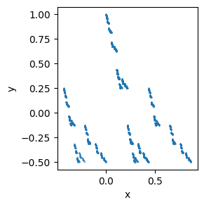
Hmm. This does not look so good. Maybe the issue is that the \(x_n\) are not uniformly distributed. Let’s use \(y_n\) instead:
Ns = 10000
y = get_uniform(Ns)
p = get_sierpinski(y)
fig, ax = plt.subplots()
ax.plot(p.real, p.imag, '.', ms=0.5)
ax.set(aspect=1, xlabel="x", ylabel="y");
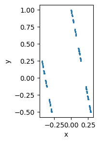
Oh dear! This is even worse! What is going on? It looks like I might have a bug in my
get_sierpinski() code, but we saw that NumPy’s random numbers worked fine. What is
going on? Please explain what is broken and try to fix it.
Hints#
# Need a hint?  Try reshaping the other way, then taking the transpose.  I.e., replace
x, y = y_.reshape((2, Ns))

# with

x, y = y_.reshape((Ns, 2)).T

# Remember that python arrays are in row-major order as in C.
# The first shape above orders these as y_ = (x0, x1, x2, ..., y0, y1, y2, ...)
# The second shape orders these as      y_ = (x0, y0, x1, y1, x2, y2, ...)
---------------------------------------------------------------------------
ValueError                                Traceback (most recent call last)
Cell In[9], line 2
      1 # Need a hint?  Try reshaping the other way, then taking the transpose.  I.e., replace
----> 2 x, y = y_.reshape((2, Ns))
      4 # with
      6 x, y = y_.reshape((Ns, 2)).T

ValueError: cannot reshape array of size 200000 into shape (2,10000)
# Here is the autocorrelation function... note, although this
# idea is important, the actual resuly shown here is a bit of
# a red herring.
from statsmodels.graphics.tsaplots import plot_acf
y = get_uniform(10000)
plot_acf(y, lags=90);
