Show code cell content
import mmf_setup; mmf_setup.nbinit()
import os
from pathlib import Path
FIG_DIR = Path(mmf_setup.ROOT) / '../Docs/_build/figures/'
os.makedirs(FIG_DIR, exist_ok=True)
import logging; logging.getLogger("matplotlib").setLevel(logging.CRITICAL)
%matplotlib inline
import numpy as np, matplotlib.pyplot as plt
try: from myst_nb import glue
except: glue = None
This cell adds /home/docs/checkouts/readthedocs.org/user_builds/iscimath-583-fractals/checkouts/latest/src to your path, and contains some definitions for equations and some CSS for styling the notebook. If things look a bit strange, please try the following:
- Choose "Trust Notebook" from the "File" menu.
- Re-execute this cell.
- Reload the notebook.
Iterated Function Systems#
Many fractals can be expressed in terms of an iterated function system (IFS) where one considers the behaviour of some mapping \(f: \mathcal{F} \mapsto \mathcal{F}\) that maps a metric space \(\mathcal{F}\) to itself. Given an initial point \(z_0\), this mapping defines the orbit of that point \((z_0, z_1, \cdots)\):
Such a sequence might converge to a limit point or diverge to infinity (which might also be considered as a limit point). Given a particular limit point \(p\), one can define the basin of attraction:
The boundary between different basins of attraction are often fractals.
Linear Maps#
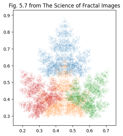
Here we discuss two types of linear map from [Barnsley et al., 1988]. The first corresponds to Fig. 5.7 and Table 5.1:
from math_583.ifs import IFS1
ifs = IFS1()
print(ifs.s)
print(ifs.a)
ax = ifs.draw(N=10000, alpha=0.1)
ax.set_title("Fig. 5.7 from The Science of Fractal Images");
[0.6+0.j  0.6+0.j  0.4-0.3j 0.4+0.3j]
[0.45+0.9j 0.45+0.3j 0.6 +0.3j 0.3 +0.3j]
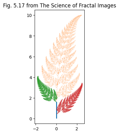
The second corresponds to Fig. 5.17 and Table 5.2:
Each entry in the trans_rots_scales table is a list of 3 tuples \([(h, k), (\theta,
\psi), (r, s)]\) with the parameters above. Note that the angles are in degrees here.
from math_583 import ifs
ifs = ifs.IFSBarnsley()
print(ifs.trans_rots_scales)
ax = ifs.draw(N=10000, ms=0.1)
ax.set_title("Fig. 5.17 from The Science of Fractal Images");
[[[  0.     0.  ]
  [  0.     0.  ]
  [  0.     0.16]]

 [[  0.     1.6 ]
  [ -2.5   -2.5 ]
  [  0.85   0.85]]

 [[  0.     1.6 ]
  [ 49.    49.  ]
  [  0.3    0.3 ]]

 [[  0.     0.44]
  [120.   -50.  ]
  [  0.3    0.37]]]
from math_583.ifs import IFS2
ifs = IFS2()
ax = ifs.draw(N=10000)
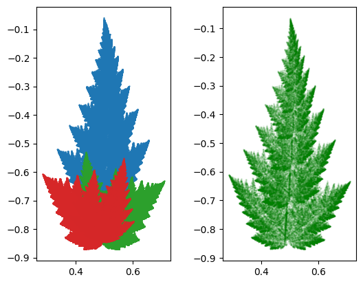
SuperFractals#
Here is a different IFS from the book [Barnsley, 2006]:
Here we draw the images on the left, and an approximation to what he refers to as the measure fractal on the right by playing the Chaos game:
from math_583.ifs import IFSSuperFractal
ifs = IFSSuperFractal(weights=[60, 0, 20, 19])
fig, axs = plt.subplots(1, 2)
ifs.draw(N=100000, ax=axs[0]);
ifs.draw(N=100000, alpha=0.1, c='g', images=False, ax=axs[1]);
Mandelbrot and Julia Sets#
Additional references:
Given an IFS \(f\) one can define the Julia set \(J_f\) as the set of points at the boundaries of the basins of attraction. One of the simplest such IFS has a single parameter \(c\):
The limit points are
In addition, iterations can diverge to the “limit point” \(p_{\infty} = \infty\).
Nx, Ny = Nxy = (256*8,)*2
Rx, Ry = Rxy = (2, 2)
Rx, Ry = Rxy = (1.5, 1.5)
x, y = [np.linspace(-R, R, N) for R, N in zip(Rxy, Nxy)]
X, Y = np.meshgrid(x, y)
Z = X + 1j*Y

R = 4  # Bailout radius

c = -1.3 + 0.03j
c = 0.365 + 0.3j
c = 0.3646 + 0.3j
d = np.sqrt(1-4*c)
p = np.array([1-d, 1+d])/2

def f(z, c):
    return z**2 + c

# Here we use sympy to compute the Newton iteration.
assert(np.allclose(f(p, c), p))  # Check that limit points are invariant

fig, ax = plt.subplots(1, 1, figsize=(10, 10*Ry/Rx))
%time for n in range(200): Z = f(Z, c)
C = np.where(np.logical_or(abs(Z) > R, np.isnan(Z)),
    -1,
    np.argmin(abs(Z[:, :, None] - p[None, None, :]), axis=-1))
ax.pcolormesh(x, y, C, shading="auto")
ax.plot(p.real, p.imag, 'rx')
ax.set(xlabel=r'$x=\Re z$', ylabel=r'$y=\Im z$',
       title=f"{c=}");
/tmp/ipykernel_3966/4169236502.py:17: RuntimeWarning: overflow encountered in square
  return z**2 + c
/tmp/ipykernel_3966/4169236502.py:17: RuntimeWarning: invalid value encountered in square
  return z**2 + c
CPU times: user 2.66 s, sys: 3.81 s, total: 6.47 s
Wall time: 6.47 s
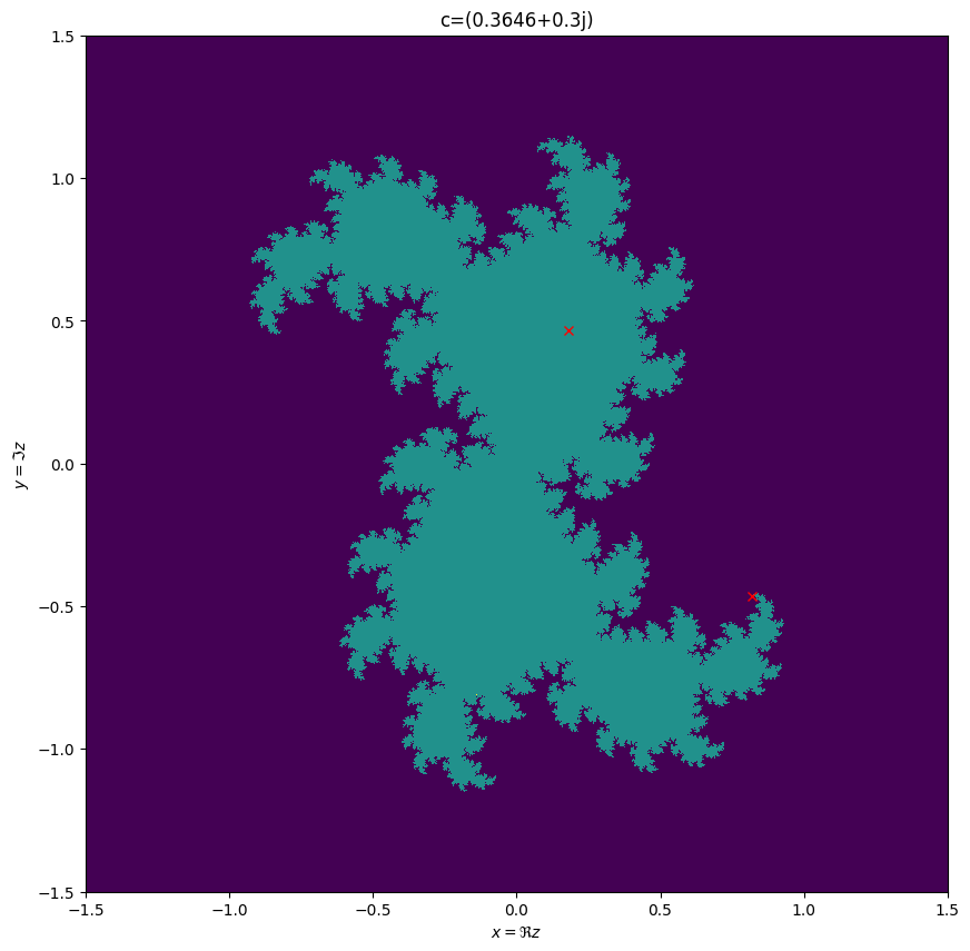
Some things to note and explore:
The interior is a single basin of attraction: one of the limit points is attractive, while the other is repulsive. These are plotted as red xs. The repulsive fixed-point is contained in the Julia set.
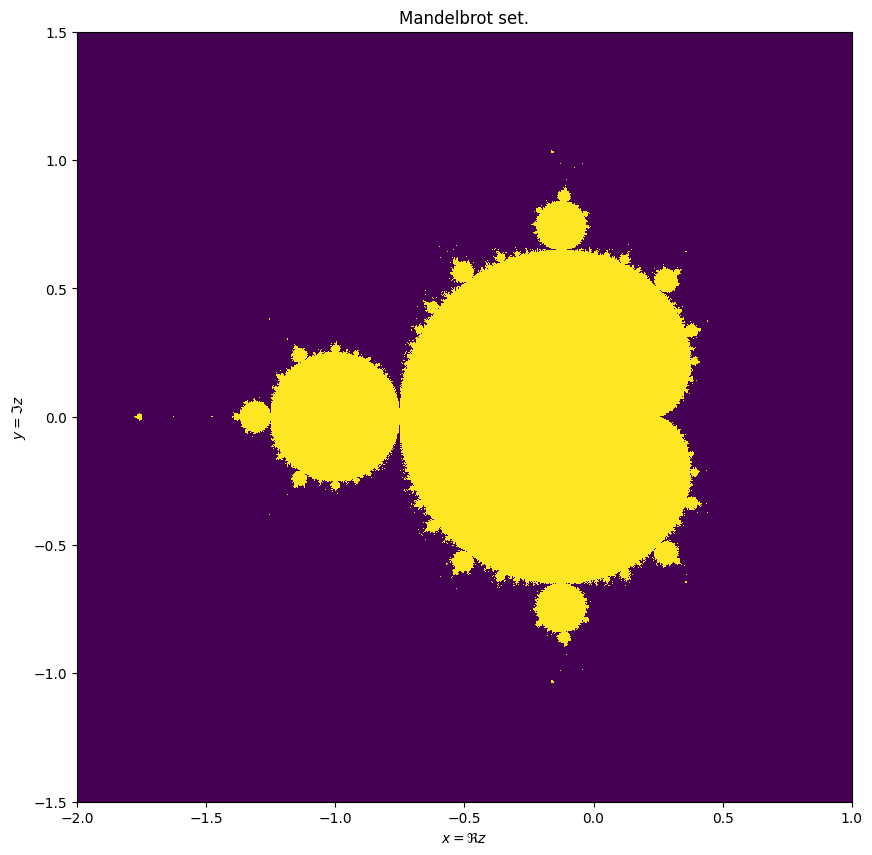
How does the shape depend on the value of \(c\)? The set of points \(c\) where the Julia set is connected is called the Mandlebrot set \(M(f)\).
If \(c\) is not in the Mandelbrot set, then the corresponding Julia set has measure zero (sometimes called Fatou dust)
How does the dimension of \(J_c\) depend on \(c\)? (Which dimension do you want to use? How can you estimate this? Can you compute it numerically?)
Note that the Julia set looks qualitatively similar everywhere, but that this qualitative nature depends on the parameter \(c\).
Due to the symmetry of the Julia sets, one can determine if \(c \in M(f)\) by testing if the origin \(z_0=0\) escapes or not.
Nx, Ny = Nxy = (256*8,)*2
Rx, Ry = Rxy = (1.5, 1.5)
x0, y0 = -0.5, 0
x, y = [np.linspace(-R, R, N) + x0 for R, N, x0 in zip(Rxy, Nxy, (x0, y0))]
X, Y = np.meshgrid(x, y)

c = X + 1j*Y
Z = 0*c

R = 4  # Bailout radius

def f(z, c):
    return z**2 + c

fig, ax = plt.subplots(1, 1, figsize=(10, 10*Ry/Rx))
%time for n in range(100): Z = f(Z, c)
C = np.where(np.logical_or(abs(Z) > R, np.isnan(Z)), 0, 1)
ax.pcolormesh(x, y, C, shading="auto")
ax.set(xlabel=r'$x=\Re z$', ylabel=r'$y=\Im z$',
       title="Mandelbrot set.");
/tmp/ipykernel_3966/3872025167.py:13: RuntimeWarning: overflow encountered in square
  return z**2 + c
/tmp/ipykernel_3966/3872025167.py:13: RuntimeWarning: invalid value encountered in square
  return z**2 + c
CPU times: user 1.93 s, sys: 1.83 s, total: 3.76 s
Wall time: 3.76 s
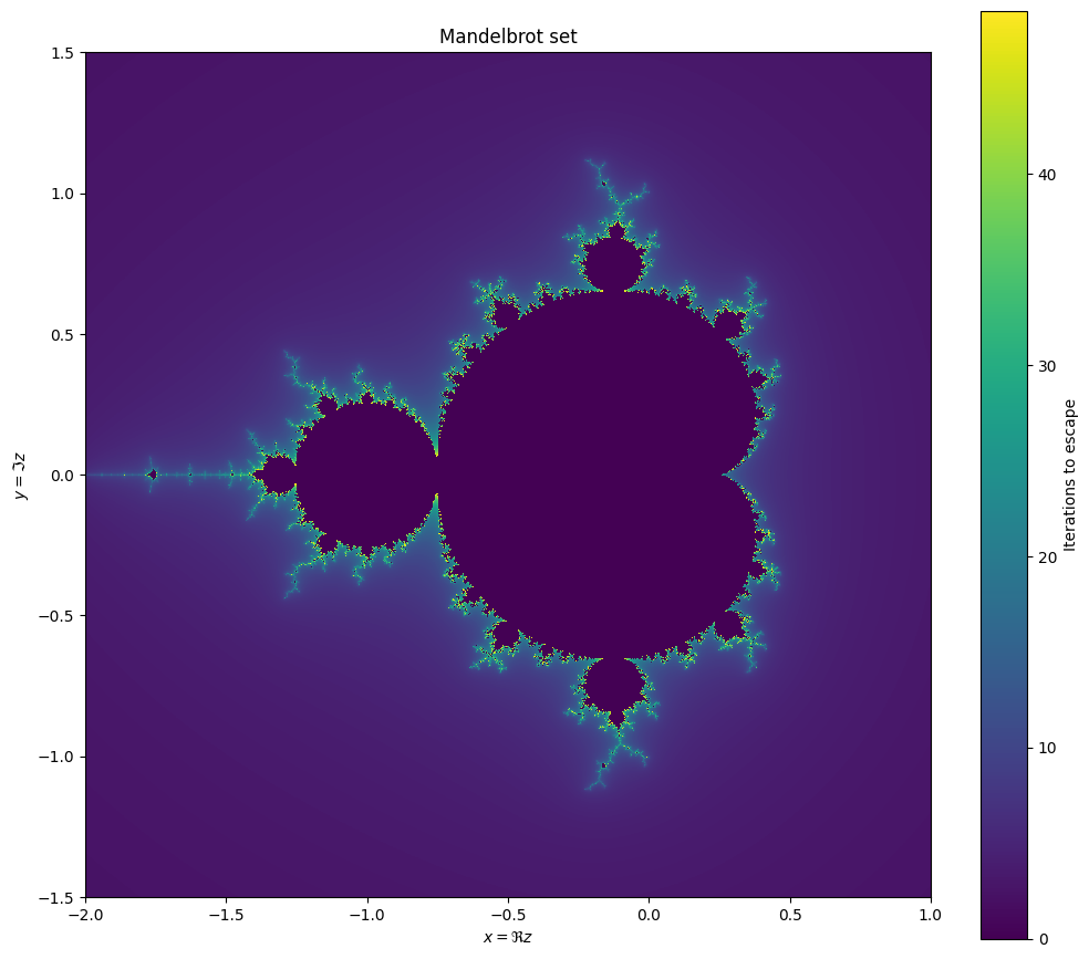
Escape-Time Algorithm#
If \(c\) is not in the Mandelbrot set, then the corresponding Julia set \(J_c\) has zero measure, and visualization using the previous techniques becomes problematic. Almost surely, the initial points will not lie in \(J_c\), hence after enough iterations, almost all the points will escape. A better way to visualize these fractals is to use the escape-time algorithm where one colours a pixel based on how many iterations it takes to “escape” (typically defined as the value of \(n\) where \(\abs{z_n} > R = 4\) for the first time).
Nx, Ny = Nxy = (256*8,)*2
Rx, Ry = Rxy = (1.5, 1.5)
x0, y0 = -0.5, 0
x, y = [np.linspace(-R, R, N) + x0 for R, N, x0 in zip(Rxy, Nxy, (x0, y0))]
X, Y = np.meshgrid(x, y)

c = X + 1j*Y
Z = 0*c

R = 16  # Bailout radius
Nmax = 100000  # Dummy value used to separate values

smooth = True

def f(z, c, n):
    z_ = abs(z)
    if smooth:
        # Correction to smoothly iterpolate colors.  See Wikipedia
        # This has an error that gets very small when R is large.
        corr = 1 - np.log(np.log(z_))/np.log(2)
    else:
        corr = 0

    return np.where(
        z_ < R,
        z**2 + c,
        np.where(z_ > Nmax, z, Nmax + n + corr))

%time for n in range(50): Z = f(Z, c, n)
C = np.where(abs(Z) > Nmax, Z - Nmax, 0).real
# plt.plot(x, C[:, 0].real)

fig, ax = plt.subplots(1, 1, figsize=(10, 10*(Ry/Rx - 0.1)))
mesh = ax.pcolormesh(x, y, C, shading="auto")
plt.colorbar(mesh, ax=ax, fraction=0.1,
             label='Iterations to escape')
ax.set(xlabel=r'$x=\Re z$', ylabel=r'$y=\Im z$',
       title="Mandelbrot set", aspect=1)
plt.tight_layout();
/tmp/ipykernel_3966/940368981.py:20: RuntimeWarning: divide by zero encountered in log
  corr = 1 - np.log(np.log(z_))/np.log(2)
/tmp/ipykernel_3966/940368981.py:20: RuntimeWarning: invalid value encountered in log
  corr = 1 - np.log(np.log(z_))/np.log(2)
CPU times: user 4.69 s, sys: 4.92 s, total: 9.6 s
Wall time: 9.61 s
R = 4
def f(z, c, n):
    z_ = abs(z)
    if smooth:
        # Correction to smoothly iterpolate between z_ = R and z_ = R**2
        corr = 1 - np.log(z_/R)/np.log(R**(2-1))
        corr = 2 - np.log(z_)/np.log(R)
        corr = 2 - np.log(z_)/np.log(R)
        corr = 1 - np.log(np.log(z_))/np.log(2)
        corr = 1 - np.log(np.log(z_))/np.log(2)
    else:
        corr = 0

    return np.where(
        z_ < R,
        z**2 + c,
        np.where(z_ >= Nmax, z, Nmax + n + corr))

c = np.linspace(-2, 2, 2000)*1j - 2
#c = np.linspace(-2, -1, 2000)*1j - 2
#c = np.linspace(-1.34, -1.32, 20)*1j - 2
Z = 0*c
%time for n in range(50): Z = f(Z, c, n)
C = np.where(abs(Z) > Nmax, Z - Nmax, 0).real
plt.clf()
plt.plot(c.imag, C)


#z_ = R, 1 - log(z_/R)/log(R)
#z_ = R**2, 1-log(z_/R)/log(R) = 0
#log(z_)z_/R = 1
#z_/R**2

%time for n in range(50): Z = f(Z, c, n)
C = np.where(abs(Z) > Nmax, Z - Nmax, 0).real
plt.plot(x, C[:, 0])

fig, ax = plt.subplots(1, 1, figsize=(10, 10*(Ry/Rx - 0.1)))
mesh = ax.pcolormesh(x, y, C, shading="auto")
plt.colorbar(mesh, ax=ax, fraction=0.1,
             label='Iterations to escape')
ax.set(xlabel=r'$x=\Re z$', ylabel=r'$y=\Im z$',
       title="Mandelbrot set", aspect=1)
plt.tight_layout();
Many fractals can be defined as the set of points which do not “escape to infinity” when a certain mapping is repeatedly applied. The famous Mandelbrot and Julia sets are defined in this way, as is the Sierpinski gasket can also be defined this way as described in the section titled Sir Pinski’s Game and Deterministic Chaos in Chapter 1 of [Schroeder, 1991].
These require a mapping \(f: \mathcal{F} \rightarrow \mathcal{F}\) (i.e. an injection) on some metric space \(\mathcal{F}\) with an origin. This mapping defines a sequence of points
The escape-time fractals are the sets of points where these sequences remain bounded as \(n \rightarrow \infty\):
Generally \(\lim_{R\rightarrow\infty} J_R(f) = J(f)\) converges and one need just choose a suitably large \(R\).
Often, the function \(z \mapsto f_c(z)\) depends on a control parameter \(c \in \mathcal{F}\). For this family of functions, the set \(J_c = J(f_c)\) depends on the parameter \(c\). A related set is
which is the set of all control parameters \(c\) for which the iterates of some initial point \(z_0\) do not escape.
This allows us to define two escape-time fractals:
do not “escape” to infinity
Generally \(\lim_{R\rightarrow\infty} M_R(f) = M(f)\) converges and one need just choose a suitably large \(R\).
Here are some well-known examples:
Mandelbrot Set: \(f(z) = z^2+c\)
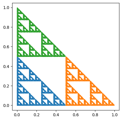
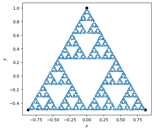
One way to define certain types of fractals is through what is called an iterated function system. Chapter 1 of [Schroeder, 1991]describes Sir Pinski’s Game and Deterministic Chaos: given three points defining an equilateral triangle,
Chapter 1: [Schroeder, 1991].
Here we play Sir Pinski’s game.
Note
To simplify the implementation, we use complex numbers \(z=x+\I y\) to represent the points. This makes it easy, for example, to define the vertices \(p_n\) of an equilateral triangle:
To plot these, we need a function z2xy() that extracts and packages the real and
imaginary parts into an appropriate array so that they can be plotted. We use a
property of NumPy arrays that allows a complex array to be viewed as a real array with
twice as many elements. We then reshape things so that the first index selects \(x\) and
\(y\).
We now iterate as follows:
where \(p_{n}\) is one of the vertices, randomly chosen.
Show code cell source
# We will work with complex numbers z = x+1j*y.
ths = np.pi/2 + 2*np.pi * np.arange(3)/ 3
ps = np.exp(1j*ths)   # Points on the triangle.
fig, ax = plt.subplots()

def z2xy(z):
    """Return (x, y) array for complex points z."""
    return np.einsum('...j->j...',
        np.asarray(z, dtype=complex).view(dtype=float).reshape(z.shape + (2,)))

# Use a properly seeded random number generator so we can reproduce our results.
rng = np.random.default_rng(seed=2)

def sirpinski(N, z0=ps[0], Nskip=0, rng=rng, fast=False):
    """Generate N points randomly moving towards the Sirpinski attractor.

    Arguments
    ---------
    N : int
        Points to generate
    z0 : complex
        Initial point
    Nskip : int
        Number of points to skip.
    """
    if fast:
        n = j = np.arange(N+Nskip)
        pj = ps[rng.integers(3, size=N+Nskip)]
        return (z0 + np.cumsum(pj*2**j))/2**n
    else:
        z = z0
        zs = []
        for n in range(Nskip+N):
            z = (z + ps[rng.integers(3)])/2
            if n > Nskip:
                zs.append(z)
        return np.asarray(zs)

ax.plot(*z2xy(ps), 'ok')
ax.plot(*z2xy(sirpinski(10000)), '.', ms=1)
ax.set(xlabel='$x$', ylabel='$y$', aspect=1);
Exercises#
Reproduce the following video from the Julia set Wikipedia page which explores \(c=0.7885e^{\I\theta}\):

