Show code cell content
import mmf_setup; mmf_setup.nbinit()
import os
from pathlib import Path
import logging
logging.getLogger("matplotlib").setLevel(logging.CRITICAL)
logging.getLogger("numba").setLevel(logging.CRITICAL)
%matplotlib inline
import numpy as np, matplotlib.pyplot as plt
This cell adds /home/docs/checkouts/readthedocs.org/user_builds/iscimath-583-fractals/checkouts/latest/src to your path, and contains some definitions for equations and some CSS for styling the notebook. If things look a bit strange, please try the following:
- Choose "Trust Notebook" from the "File" menu.
- Re-execute this cell.
- Reload the notebook.
Percolation#
Here we discuss Chapter 15 in [Schroeder, 1991]: Percolation: From Forest Fires to Epidemics and [Albinet et al., 1986], which discusses a model for forest fires. The model is that trees randomly populate the sites of a square lattice with probability \(p\). If a tree is on fire at time \(t\), then any tree occupying one of the 4 nearest neighboring sites (sometimes called the von Neumann neighbourhood) will burn at time \(t+1\).
They start by igniting all trees in the top row (\(n=0\)). Some details and code are provided in HPC Assignment 1: Percolation. We use that code here to demonstrate burning of a 100×100 lattice at the percolation threshold \(p=p_c \approx 0.592\):
Show code cell source
from itertools import product
from matplotlib.colors import ListedColormap
from numba import njit, prange
from mmfutils.plot.animation import MyFuncAnimation
from IPython.display import HTML

# 0: No tree
# 1: Living tree
# 2: Burning tree
# 3: Burnt tree

# Some plotting routines
cm = ListedColormap(["black", "green", "red", "grey"])
def draw(X, ax=None):
    if ax is None:
        ax = plt.gca()
    ax.imshow(X, origin='lower', interpolation='none',
              cmap=cm, vmin=0, vmax=3)
    ax.set(aspect=1, ylabel='$n$')

@njit(parallel=True)
def update(X_):
    Nx, Ny = X_[1:-1, 1:-1].shape
    X1_ = X_.copy()
    for nx in prange(1, Nx+1):
        for ny in range(1, Ny+1):
            if X_[nx, ny] == 2:  # If tree is on fire
                 X1_[nx, ny] = 3  # New tree is burnt.
            elif (X_[nx, ny] == 1
                and (X_[nx-1, ny] == 2
                     or X_[nx+1, ny] == 2
                     or X_[nx, ny-1] == 2
                     or X_[nx, ny+1] == 2)):
                 X1_[nx, ny] = 2
    # Periodic boundaries
    for nx in prange(1, Nx+1):
        X1_[nx, 0] = X1_[nx, -2]
        X1_[nx, -1] = X1_[nx, 1]
    return X1_

def evolve(Nxy=(100, 100), p=0.5927460507921, seed=3):
    """Return the stages `X_` until the fire goes out."""
    Nx, Ny = Nxy
    rng = np.random.default_rng(seed=seed)
    X = rng.choice(2, size=Nxy, p=[1-p, p])

    # Make slightly large array to add ghost-points to simplify testing
    X_ = np.zeros((Nx+2, Ny+2))
    X_[1:-1, 1:-1] = X

    # Periodic boundary conditions
    X_[:, 0] = X_[:, -2]
    X_[:, -1] = X_[:, 1]

    # Burning top row
    X_[1, :] *= 2

    Xs = [X_[1:-1, 1:-1].copy()]
    while np.any(X_[1:-1, 1:-1] == 2):
        X_ = update(X_)
        Xs.append(X_[1:-1, 1:-1].copy())

    return np.asarray(Xs)

def get_frames(Xs, ax):
    fig = ax.figure

    # Initial frame used to setup the figure.
    # This is not recorded in the movie.
    X = Xs[0]
    draw(X, ax=ax)
    yield fig

    yield fig
    for X in Xs[1:]:
        ax.cla()
        draw(X, ax=ax)
        yield fig

Nxy = (100, 200)
p = 0.5927460507921

%time Xs = evolve(Nxy=Nxy, p=p)
fig, ax = plt.subplots(figsize=(6, 3))
anim = MyFuncAnimation(
    fig=fig,
    func=lambda frame:frame,
    frames=get_frames(Xs=Xs, ax=ax),
    interval=20)
plt.close('all')
HTML(anim.to_html5_video())
CPU times: user 1.15 s, sys: 71.5 ms, total: 1.23 s
Wall time: 1.14 s
Power-laws#
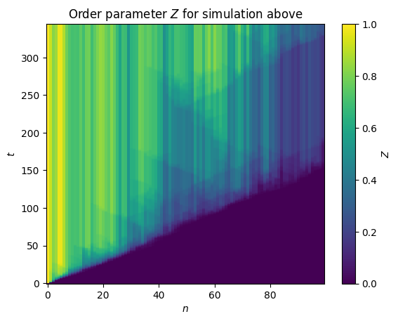
Consider a lattice of length (left-to-right) \(L\). The average number of trees in each row is thus \(pL\). The paper [Albinet et al., 1986] defines the order parameter \(Z(n, t, \epsilon)\) to be the number of burned trees in row \(n\) at time-step \(t\) divided by \(pL\):
Nx, L =  Nxy
def get_Z(Xs, p):
    Nt, Nx, L = Xs.shape
    Z = (Xs==3).sum(axis=-1) / (p*L)
    return Z

ns = np.arange(Nx)
ts = np.arange(len(Xs))
fig, ax = plt.subplots()
mesh = ax.pcolormesh(ns, ts, get_Z(Xs, p=p), vmin=0, vmax=1, shading="nearest")
ax.set(xlabel="$n$", ylabel="$t$",
       title="Order parameter $Z$ for simulation above")
fig.colorbar(mesh, ax=ax, label="$Z$");
Here we average over 100 realizations:
Ns = 100
%time Zs = [get_Z(evolve(seed=2+n, Nxy=Nxy, p=p), p=p) for n in range(Ns)]

Nt = max(len(Z) for Z in Zs)
Z_ = np.zeros((Nt, Nx))
for Z in Zs:
    T = len(Z)
    Z_[:T, :] += Z
    Z_[T:, :] += Z[-1, :]  # Fill remaining times with last time.
Z_ /= Ns

fig, ax = plt.subplots()
ts = np.arange(Nt)
mesh = ax.pcolormesh(ns, ts, Z_, vmin=0, vmax=1, shading="nearest")
ax.set(xlabel="$n$", ylabel="$t$",
       title=f"Average order parameter $Z$ for {Ns=} simulations")
fig.colorbar(mesh, ax=ax, label="$Z$");
CPU times: user 7.97 s, sys: 1.13 s, total: 9.1 s
Wall time: 4.95 s

Scaling Analysis#
The “universality postulate” states that near the critical point \(p\approx p_c\), or \(\abs{\epsilon} \ll 1\), we should expect self-similar behaviour. Such self-similarity manifests as the function \(Z\) being homogeneous here:
This homogeneous behavior is expected where \(n, t \gg 1\) (i.e. after the burn front is well developed and away from the initial starting line) and \(\epsilon \approx 0\). We will now restrict our discussion to this region and consider the constraints on \(Z(n, t, \epsilon)\) when this scaling is exact.
The assumption of this scaling form allows one to perform a type of “dimensional analysis”. In particular, the following quantities all “scale like” \(λ\):
From these, we can form three independent ratios that are “dimensionless”.
Geometric Picture.
The geometric picture and justification of this “dimensional analysis” is thus. Consider points \(\vect{x} = (n, t, \epsilon, Z) \in \mathbb{R}^4\). A given order parameter \(Z = Z(n, t, \epsilon)\) defines a 3D subsets (slices) in this space \(\mathcal{Z} \subset \mathcal{R}^4\). If you think of \(\mathbb{R}^4 = \mathbb{R}^3 \times \mathbb{R}\), then you can think of \(Z: \mathcal{R}^3 \mapsto \mathcal{R}\) as a function over the domain \((n, t, \epsilon) \in \mathcal{R}^3\), but our discussion allows for more complicated shapes (i.e. multiple branches).
The scaling defines a 1D flow through \(\mathbb{R}^4\)
This defines a foliation of \(\mathcal{R}^4\) into a set of fibers \(\{\vect{x}(λ) \mid λ \in \mathcal{R}^+ = (0, \infty)\}\). Note that these fibers also foliate \(\mathcal{Z}\): if one point \(\vect{x}(1) \in \mathcal{Z}\), then all points in the fiber \(\vect{x}(λ) \in \mathcal{Z}\).
The scaling assumption requires this behaviour no matter what the form of \(\mathcal{Z}\), and so is “trivial” in some sense. To describe the non-trivial properties of \(\mathcal{Z}\), and therefore of the percolation problem, we must look at how \(\mathcal{Z}\) changes as we move from one fiber to another.
Back to the idea of “dimensional analysis”: We can think of the parameter \(λ\) as defining a “ruler” or scale at which we are examining the system. Thus we can think of \(λ = 1\) meaning that we measure \(n\) in units of meters. If we change units to millimeters, then the numerical value of \(n\) will change by a factor of \(λ^{a_n} = 1000\). This change does not have any physical meaning, however, near the critical point because if we change the units that we measure time in by a factor of \(λ^{a_t} = 1000^{a_t/a_n}\), the units we measure \(\epsilon\) in by a factor of \(λ^{a_\epsilon}\) and the units we measure \(Z\) in by a factor of \(λ\), then everything should look the same (self-similarity).
Thus, all of the qualitative properties of the system should depend only on “dimensionless quantities” which are invariant under the scaling flow. These quantities can be expressed as appropriate ratio of the parameters as we do in the main text.
Note that, if we were to introduce as parameters \(q = n^{1/a_n}\), \(r = t^{1/a_t}\), and \(s = \epsilon^{1/a_\epsilon}\), then the \(Z_1(q, r, s) = Z(n, t, \epsilon)\) would be a homogeneous function of degree \(1\):
This is exactly the same as the notion of extensivity in thermodynamics where the energy \(U\) of a system is a homogeneous function of the extensive entropy \(S\), volume \(V\), particle number \(N\), etc.:
Here \(λ\) denotes changes to the size of the system.
Euler’s homogeneous function theorem, which can be derived by computing the derivative at \(λ=1\), gives:
The partial derivatives give the corresponding potentials – the temperature \(T\), pressure \(P\), chemical potential \(\mu\), etc. – which are intensive quantities, independent of the system size.
A similar generalized relationship holds for us
The manipulations here to derive various relationships are in this way directly analogous to the manipulations performed in classical thermodynamics (Maxwell relations etc.). For a more detailed geometric picture in terms of a contact bundle in \(\mathcal{R}^{2n+1=7}\), with a contact ideal generated by the 1-form
see [Burke, 1985].
For example:
The general solution can then be expressed in terms of an arbitrary function of these:
Up to subtleties with invertibility, we can solve for \(\tilde{Z}\) and write \(\tilde{Z} = g(\tilde{n}, \tilde{t})\):
This clearly has the homogeneous scaling property.
Do it! Show that this form satisfies the scaling properties.
Write the scaling property as
Now use the previous relationship:
Notice that all of the scaling factors cancel in the last expression, so this is obviously true.
Do it! Find the explicit form of \(Z(n)\) if \(λ Z(x) = Z(λ^a x)\).
One way of solving this is substitute \(x=1\), then let \(n = λ^{a}\), \(λ = n^{1/a}\):
where \(Z(1) = Z/n^{1/a}\) is a constant:
One can think of \(λ\) as a “ruler”, defining the scale at which we view the system. Both \(Z\) and \(n^{1/a}\) have the same “dimensions” or “units” in terms of this ruler. The universality postulate is that, near the critical point/phase transition etc., the system is scale-invariance. I.e. changing the scale simply changes the ruler \(λ\), but does not change any of the “physical properties” of the system once everything is properly adjusted.
Said in the language of dimensional analysis, the non-trivial physics should depend only on a dimensionless function of all independent dimensionless parameters. In this case:
Another approach is to differentiate with respect to \(λ\), then set \(λ = 1\):
This differential equation is separable and can be easily solved:
Do it! Find \(Z(n, t)\) if \(λ Z(x, y) = Z(λ^a x, λ^b y)\).
Similar to before, let \(x\) and \(y\) be constants, and call \(n = \lambda^a x\) and \(t = \lambda^b y\) where \(\lambda\) defines our “units”. We now have
where \(Z(x, y)\) is a constant. Thus, in the language of dimensional analysis, we say that \(n^{1/a}\), \(t^{1/b}\) and \(Z\) all have the same dimension. There are thus two independent dimensionless ratios and we should be able to express the general solution in terms of an arbitrary function of two of these. E.g.:
Limited only by potential issues of invertibility we can solve for either quantity, and express
so the general solution in most cases can be expressed as:
where \(f\) is an arbitrary function.
Percolation Threshold and Critical Exponents#
If we knew the critical exponents, then we could use these relationships to “collapse” the data to a lower-dimensional manifold. We first demonstrate this by cheating again with the extracted exponents from [Albinet et al., 1986]:
Since we have data above for \(\epsilon = 0\), we should choose a different parameterization introducing the function \(z_1(t/n^{a_t/a_n})\) from [Albinet et al., 1986]::
beta = 0.12
tau = 1.55
nu = 0.87 * tau

a_n = -nu/beta
a_t = -tau/beta
a_e = 1/beta
print(f"{a_n=:.2f}, {a_t=:.2f}, {a_e=:.2f}");

n_, t_ = np.meshgrid(ns, ts)

with np.errstate(all='ignore'):
    z1 = Z_ / n_**(1/a_n)
    x = t_/n_**(a_t/a_n)
fig, ax = plt.subplots()
ax.loglog(x.ravel(), z1.ravel(), '.', alpha=0.1)
ax.loglog(x[10:, 10:].ravel(), z1[10:, 10:].ravel(), '.')
ax.set(xlabel="$t/n^{a_t/a_n}$", ylabel="$z_1 = Z/n^{1/a_n}$", xlim=(0.5, 300),
       title=f"Universal function $Z/n^{{{1/a_n=:.2g}}} = z_1(t/n^{{{a_t/a_n=:.2g}}})$");
a_n=-11.24, a_t=-12.92, a_e=8.33

However, we must first determine the critical exponents and the percolation threshold \(p_c\). This is the point of most of the discussion in [Albinet et al., 1986]. To compute \(p_c\), they suggest looking at the “probability of penetration” \(P\): i.e. the probability that a path connects the bottom and top of the lattice. They argue that at \(p_c\) this, should be independent of the lattice size \(L\), and so can be computed for small lattices.
# Figure 3.
# This cell takes a couple of minutes to run as it accumulates statistics
Ls = [20, 40, 80, 100]
Ns = 200
pc = 0.5927460507921
ps = np.linspace(0.45, 0.7, 20)

burn_throughs = np.zeros((len(Ls), len(ps)), dtype=int)
burn_times = np.zeros((len(Ls), len(ps)), dtype=int)

for n in range(Ns):
    for i, L in enumerate(Ls):
        for j, p in enumerate(ps):
            Xs = evolve(Nxy=(L, L), p=p, seed=2+n)
            burn_throughs[i, j] += np.any(Xs[-1][-1, :] == 3)
            burn_times[i, j] += len(Xs)
            del Xs
burn_throughs = burn_throughs / Ns
burn_times = burn_times / Ns

fig, ax = plt.subplots()
lines = ax.plot(ps, burn_throughs.T, '+-')
ax.legend(labels=[f"{L=}" for L in Ls])
ax.set(ylim=(0,1), xlabel="$p_c$", ylabel="$P$", title=f"Fig.3: {Ns=} samples")
ax.axvline(pc, c='y', ls=':');

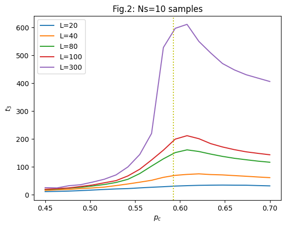
# Figure 2.

L = 300
Ns = 10

%time Ts = [np.mean([len(evolve(Nxy=(L, L), p=p, seed=2+n)) for n in range(Ns)]) for p in ps]

fig, ax = plt.subplots()
ax.plot(ps, burn_times.T)
ax.plot(ps, Ts)
ax.set(xlabel="$p_c$", ylabel="$t_3$", title=f"Fig.2: {Ns=} samples")
ax.legend(labels=[f"{L=}" for L in Ls + [L]])
ax.axvline(pc, c='y', ls=':');
CPU times: user 1min 10s, sys: 25.9 s, total: 1min 35s
Wall time: 55.3 s
[Albinet et al., 1986]#
For reasons that we will just say are conventional for now, the paper expresses the powers \(a_n\), \(a_t\), and \(a_\epsilon\) in terms of some different parameters:
In terms of these, we have
etc. The quantities in parentheses are simplified quantities that are “scale invariant”, and these form the basis for the remaining analysis. Note that the last two relations suggest that \(\xi \propto e^{-\nu}\) is a natural “length scale” or correlation length while \(\theta \propto e^{-\tau}\) forms a natural “time scale” or characteristic time.
Thus, equations (2.4), (2.5), and (2.8) can simply be thought of as natural scale-invariant relationships: \(Z/n^{-\beta \nu}\) and \(Z/\epsilon^{\beta}\) are scale-invariant, and thus must be a “dimensionless” function of two other independent scale-invariant quantities. We can express this in different ways, with two different forms \(f()\) and \(h()\):
Eq. (2.5) formally comes from considering the \(\epsilon \rightarrow 0\) limit while Eq. (2.9) comes from considering the infinite-time limit \(t\rightarrow\infty\) (i.e, what the burned forest looks like after the fire has burnt itself out). To apply this to Eq. (2.4) would require some limiting or asymptotic form of \(f()\), hence we introduce a scale-invariant quantity that is independent of \(\epsilon\) in \(h()\):
The discussion below Eq. (2.9) identifies the percolation threshold - i.e. how many burned trees are there at the top row \(n=L \rightarrow \infty\):
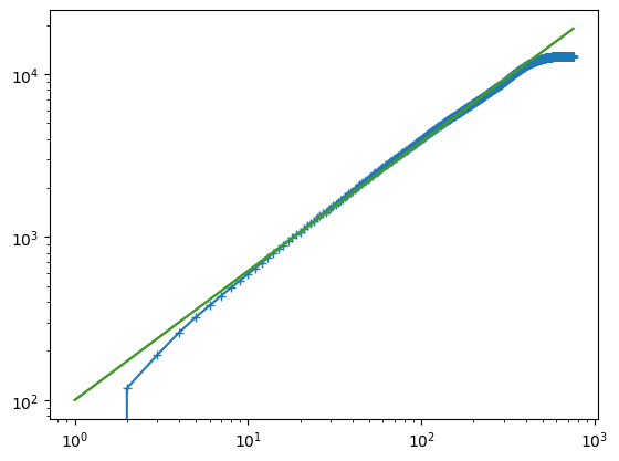
Another metric introduced in the paper is the total number of burned trees \(N_b\):
This is the basis for Fig. 4b from which the exponent \((\nu - \beta)/\tau = (1+a_n)/a_t = 0.79(2)\) is extracted.
# Figure 4b

# This cell takes about 10s to run with Ns=50.  The paper uses 300 which takes about
Ns = 50
Nx, Ny = Nxy = (200, 200)
p = pc
%time Nbs = [(evolve(seed=2+n, Nxy=Nxy, p=p) == 3).sum(axis=(-1, -2)) for n in range(Ns)]
Nt = max(len(Nb) for Nb in Nbs)
ts = 1+np.arange(Nt)
Nb_ = np.zeros(Nt)
for Nb in Nbs:
    Nb_[:len(Nb)] += Nb
    Nb_[len(Nb):] += Nb[-1]  # Fill remaining times with last time.
Nb_ /= Ns
del Nbs

beta = 0.12
tau = 1.55
nu = 0.87 * tau
#beta = 5/36
#nu = 4/3

a_n = -nu/beta
a_t = -tau/beta
a_e = 1/beta

plt.loglog(ts, Nb_, '-+')
plt.plot(ts, 100*ts**((nu-beta)/tau))
plt.plot(ts, 100*ts**((1+a_n)/a_t))
CPU times: user 10.5 s, sys: 1.12 s, total: 11.6 s
Wall time: 7 s
[<matplotlib.lines.Line2D at 0x7f96fbf45990>]
References:#
[Schroeder, 1991]: Chapter 15 – Percolation: From Forest Fires to Epidemics
[Albinet et al., 1986]: Ref. [ASS 86] in [Schroeder, 1991].
[Stauffer and Aharony, 1994]: Revised 2nd Edition of Ref. [Sta 85] in [Schroeder, 1991].